Month: August 2017
Running the PhysiCell sample projects
Introduction
In PhysiCell 1.2.1 and later, we include four sample projects on cancer heterogeneity, bioengineered multicellular systems, and cancer immunology. This post will walk you through the steps to build and run the examples.
If you are new to PhysiCell, you should first make sure you’re ready to run it. (Please note that this applies in particular for OSX users, as Xcode’s g++ is not compatible out-of-the-box.) Here are tutorials on getting ready to Run PhysiCell:
- Setting up a 64-bit gcc environment in Windows.
- Setting up gcc / OpenMP on OSX (MacPorts edition)
- Setting up gcc / OpenMP on OSX (Homebrew edition)
Note: This is the preferred method for Mac OSX. - Getting started with a PhysiCell Virtual Appliance (for virtual machines like VirtualBox)
Note: The “native” setups above are preferred, but the Virtual Appliance is a great “plan B” if you run into trouble
Please note that we expect to expand this tutorial.
Building, running, and viewing the sample projects
All of these projects will create data of the following forms:
- Scalable vector graphics (SVG) cross-section plots through z = 0.0 μm at each output time. Filenames will look like snapshot00000000.svg.
- Matlab (Level 4) .mat files to store raw BioFVM data. Filenames will look like output00000000_microenvironment0.mat (for the chemical substrates) and output00000000_cells.mat (for basic agent data).
- Matlab .mat files to store additional PhysiCell agent data. Filenames will look like output00000000_cells_physicell.mat.
- MultiCellDS .xml files that give further metadata and structure for the .mat files. Filenames will look like output00000000.xml.
You can read the combined data in the XML and MAT files with the read_MultiCellDS_xml function, stored in the matlab directory of every PhysiCell download. (Copy the read_MultiCellDS_xml.m and set_MultiCelLDS_constants.m files to the same directory as your data for the greatest simplicity.)
(If you are using Mac OSX and PhysiCell version > 1.2.1, remember to set the PHYSICELL_CPP environment variable to be an OpenMP-capable compiler – rf. Homebrew setup.)
Biorobots (2D)
Type the following from a terminal window in your root PhysiCell directory:
make biorobots-sample
make
./biorobots
make reset # optional -- gets a clean slate to try other samples
Because this is a 2-D example, the SVG snapshot files will provide the simplest method of visualizing these outputs. You can use utilities like ImageMagick to convert them into other formats for publications, such as PNG or EPS.
Anti-cancer biorobots (2D)
make cancer-biorobots-sample
make
./cancer_biorobots
make reset # optional -- gets a clean slate to try other samples
Cancer heterogeneity (2D)
make heterogeneity-sample
make project
./heterogeneity
make reset # optional -- gets a clean slate to try other samples
Cancer immunology (3D)
make cancer-immune-sample
make
./cancer_immune_3D
make reset # optional -- gets a clean slate to try other samples
A small computational thought experiment
In Macklin (2017), I briefly touched on a simple computational thought experiment that shows that for a group of homogeneous cells, you can observe substantial heterogeneity in cell behavior. This “thought experiment” is part of a broader preview and discussion of a fantastic paper by Linus Schumacher, Ruth Baker, and Philip Maini published in Cell Systems, where they showed that a migrating collective homogeneous cells can show heterogeneous behavior when quantitated with new migration metrics. I highly encourage you to check out their work!
In this blog post, we work through my simple thought experiment in a little more detail.
Note: If you want to reference this blog post, please cite the Cell Systems preview article:
P. Macklin, When seeing isn’t believing: How math can guide our interpretation of measurements and experiments. Cell Sys., 2017 (in press). DOI: 10.1016/j.cells.2017.08.005
The thought experiment
Consider a simple (and widespread) model of a population of cycling cells: each virtual cell (with index i) has a single “oncogene” \( r_i \) that sets the rate of progression through the cycle. Between now (t) and a small time from now ( \(t+\Delta t\)), the virtual cell has a probability \(r_i \Delta t\) of dividing into two daughter cells. At the population scale, the overall population growth model that emerges from this simple single-cell model is:
\[\frac{dN}{dt} = \langle r\rangle N, \]
where \( \langle r \rangle \) the mean division rate over the cell population, and N is the number of cells. See the discussion in the supplementary information for Macklin et al. (2012).
Now, suppose (as our thought experiment) that we could track individual cells in the population and track how long it takes them to divide. (We’ll call this the division time.) What would the distribution of cell division times look like, and how would it vary with the distribution of the single-cell rates \(r_i\)?
Mathematical method
In the Matlab script below, we implement this cell cycle model as just about every discrete model does. Here’s the pseudocode:
t = 0;
while( t < t_max )
    for i=1:Cells.size()
        u = random_number();
        if( u < Cells[i].birth_rate * dt )
            Cells[i].division_time = Cells[i].age;
            Cells[i].divide();
        end
    end
    t = t+dt;
end
That is, until we’ve reached the final simulation time, loop through all the cells and decide if they should divide: For each cell, choose a random number between 0 and 1, and if it’s smaller than the cell’s division probability (\(r_i \Delta t\)), then divide the cell and write down the division time.
As an important note, we have to track the same cells until they all divide, rather than merely record which cells have divided up to the end of the simulation. Otherwise, we end up with an observational bias that throws off our recording. See more below.
The sample code
You can download the Matlab code for this example at:
http://MathCancer.org/files/matlab/thought_experiment_matlab(Macklin_Cell_Systems_2017).zip
Extract all the files, and run “thought_experiment” in Matlab (or Octave, if you don’t have a Matlab license or prefer an open source platform) for the main result.
All these Matlab files are available as open source, under the GPL license (version 3 or later).
Results and discussion
First, let’s see what happens if all the cells are identical, with \(r = 0.05 \textrm{ hr}^{-1}\). We run the script, and track the time for each of 10,000 cells to divide. As expected by theory (Macklin et al., 2012) (but perhaps still a surprise if you haven’t looked), we get an exponential distribution of division times, with mean time \(1/\langle r \rangle\):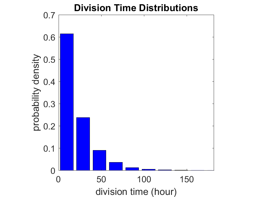
So even in this simple model, a homogeneous population of cells can show heterogeneity in their behavior. Here’s the interesting thing: let’s now give each cell its own division parameter \(r_i\) from a normal distribution with mean \(0.05 \textrm{ hr}^{-1}\) and a relative standard deviation of 25%: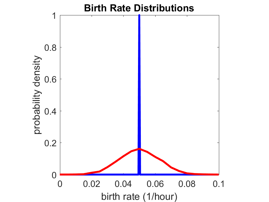
If we repeat the experiment, we get the same distribution of cell division times!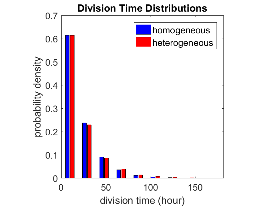
So in this case, based solely on observations of the phenotypic heterogeneity (the division times), it is impossible to distinguish a “genetically” homogeneous cell population (one with identical parameters) from a truly heterogeneous population. We would require other metrics, like tracking changes in the mean division time as cells with a higher \(r_i\) out-compete the cells with lower \(r_i\).
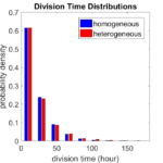
Lastly, I want to point out that caution is required when designing these metrics and single-cell tracking. If instead we had tracked all cells throughout the simulated experiment, including new daughter cells, and then recorded the first 10,000 cell division events, we would get a very different distribution of cell division times: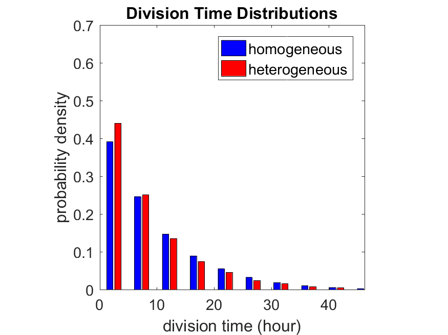
By only recording the division times for the cells that have divided, and not those that haven’t, we bias our observations towards cells with shorter division times. Indeed, the mean division time for this simulated experiment is far lower than we would expect by theory. You can try this one by running “bad_thought_experiment”.
Further reading
This post is an expansion of our recent preview in Cell Systems in Macklin (2017):
P. Macklin, When seeing isn’t believing: How math can guide our interpretation of measurements and experiments. Cell Sys., 2017 (in press). DOI: 10.1016/j.cells.2017.08.005
And the original work on apparent heterogeneity in collective cell migration is by Schumacher et al. (2017):
L. Schumacher et al., Semblance of Heterogeneity in Collective Cell Migration. Cell Sys., 2017 (in press). DOI: 10.1016/j.cels.2017.06.006
You can read some more on relating exponential distributions and Poisson processes to common discrete mathematical models of cell populations in Macklin et al. (2012):
P. Macklin, et al., Patient-calibrated agent-based modelling of ductal carcinoma in situ (DCIS): From microscopic measurements to macroscopic predictions of clinical progression. J. Theor. Biol. 301:122-40, 2012. DOI: 10.1016/j.jtbi.2012.02.002.
Lastly, I’d be delighted if you took a look at the open source software we have been developing for 3-D simulations of multicellular systems biology:
http://OpenSource.MathCancer.org
And you can always keep up-to-date by following us on Twitter: @MathCancer.
Getting started with a PhysiCell Virtual Appliance
Note: This is part of a series of “how-to” blog posts to help new users and developers of BioFVM and PhysiCell. This guide is for for users in OSX, Linux, or Windows using the VirtualBox virtualization software to run a PhysiCell virtual appliance.
These instructions should get you up and running without needed to install a compiler, makefile capabilities, or any other software (beyond the virtual machine and the PhysiCell virtual appliance). We note that using the PhysiCell source with your own compiler is still the preferred / ideal way to get started, but the virtual appliance option is a fast way to start even if you’re having troubles setting up your development environment.
What’s a Virtual Machine? What’s a Virtual Appliance?
A virtual machine is a full simulated computer (with its own disk space, operating system, etc.) running on another. They are designed to let a user test on a completely different environment, without affecting the host (main) environment. They also allow a very robust way of taking and reproducing the state of a full working environment.
A virtual appliance is just this: a full image of an installed system (and often its saved state) on a virtual machine, which can easily be installed on a new virtual machine. In this tutorial, you will download our PhysiCell virtual appliance and use its pre-configured compiler and other tools.
What you’ll need:
- VirtualBox: This is a free, cross-platform program to run virtual machines on OSX, Linux, Windows, and other platforms. It is a safe and easy way to install one full operating (a client system) on your main operating system (the host system). For us, this means that we can distribute a fully working Linux environment with a working copy of all the tools you need to compile and run PhysiCell. As of August 1, 2017, this will download Version 5.1.26.
- Download here: https://www.virtualbox.org/wiki/Downloads
- PhysiCell Virtual Appliance: This is a single-file distribution of a virtual machine running Alpine Linux, including all key tools needed to compile and run PhysiCell. As of July 31, 2017, this will download PhysiCell 1.2.2 with g++ 6.3.0.
- Download here: https://sourceforge.net/projects/physicell/files/PhysiCell/
- (Browse to a version of PhysiCell, and download the file that ends in “.ova”.)
- Version 1.2.0: http://bit.ly/2vY51P1 [sf.net]
- Download here: https://sourceforge.net/projects/physicell/files/PhysiCell/
- A computer with hardware support for virtualization: Your CPU needs to have hardware support for virtualization (almost all of them do now), and it has to be enabled in your BIOS. Consult your computer maker on how to turn this on if you get error messages later.
Main steps:
1) Install VirtualBox.
Double-click / open the VirtualBox download. Go ahead and accept all the default choices. If asked, go ahead and download/install the extensions pack.
2) Import the PhysiCell Virtual Appliance
Go the “File” menu and choose “Import Virtual Appliance”. Browse to find the .ova file you just downloaded.
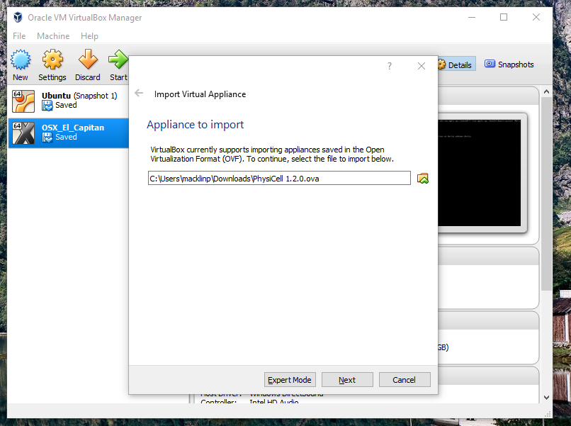
Click on “Next,” and import with all the default options. That’s it!
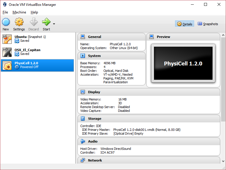
3) [Optional] Change settings
You most likely won’t need this step, but you can increase/decrease the amount of RAM used for the virtual machine if you select the PhysiCell VM, click the Settings button (orange gear), and choose “System”: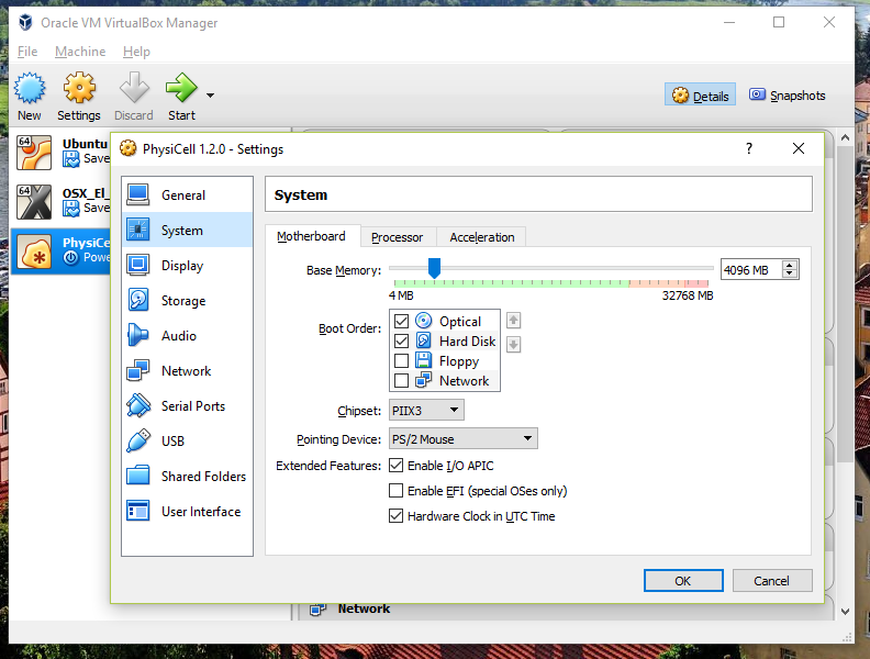 We set the Virtual Machine to have 4 GB of RAM. If you have a machine with lots of RAM (16 GB or more), you may want to set this to 8 GB.
Also, you can choose how many virtual CPUs to give to your VM: 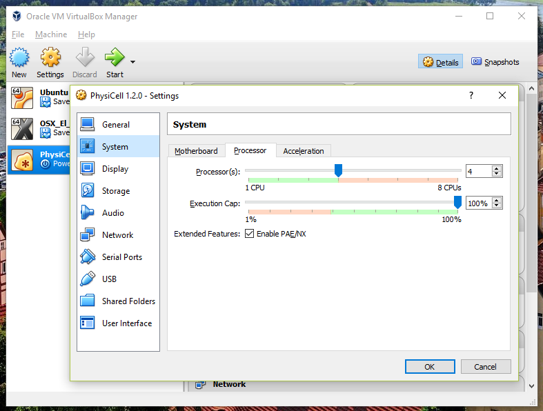
We selected 4 when we set up the Virtual Appliance, but you should match the number of physical processor cores on your machine. In my case, I have a quad core processor with hyperthreading. This means 4 real cores, 8 virtual cores, so I select 4 here.
4) Start the Virtual Machine and log in
Select the PhysiCell machine, and click the green “start” button. After the virtual machine boots (with the good old LILO boot manager that I’ve missed), you should see this: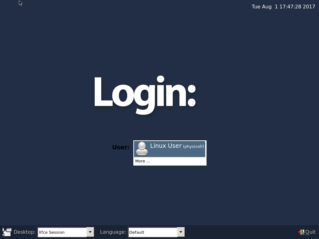
Click the "More ..." button, and log in with username: physicell, password: physicell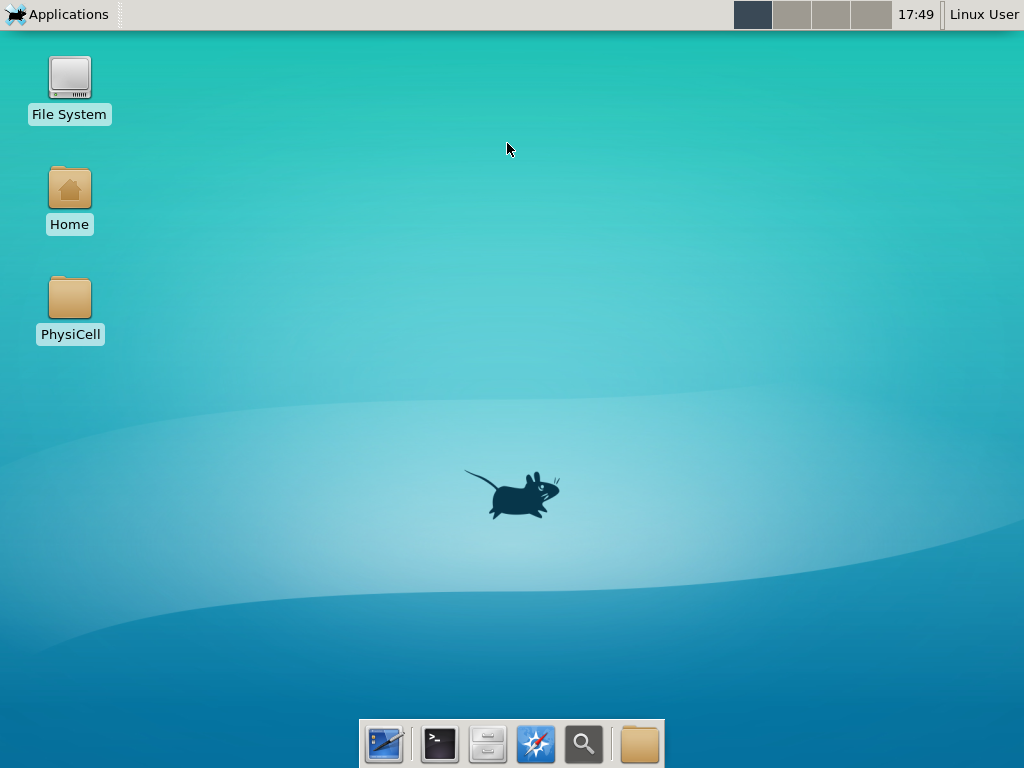
5) Test the compiler and run your first simulation
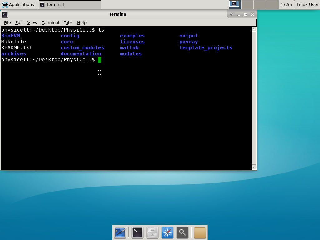
Notice that PhysiCell is already there on the desktop in the PhysiCell folder. Right-click, and choose “open terminal here.” You’ll already be in the main PhysiCell root directory. 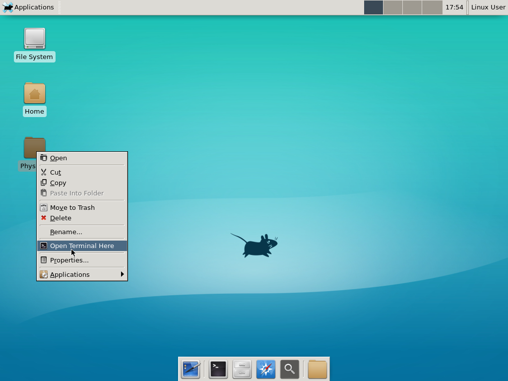
Now, let’s compile your first project! Type “make template2D && make” 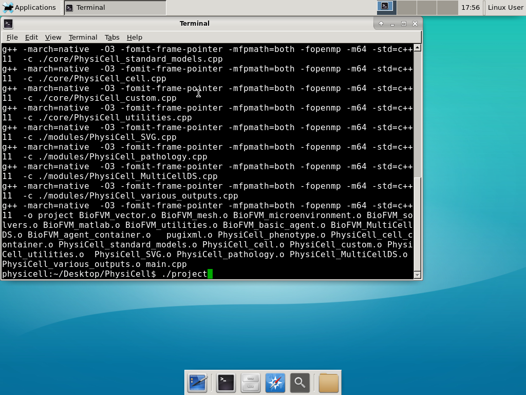 And run your project! Type “./project” and let it go!
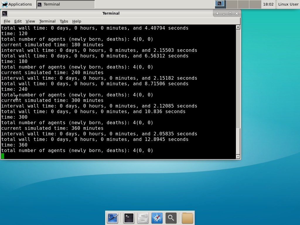 Go ahead and run either the first few days of the simulation (until about 7200 minutes), then hit <control>-C to cancel out. Or run the whole simulation–that’s fine, too.
6) Look at the results
We bundled a few tools to easily look at results. First, ristretto is a very fast image viewer. Let’s view the SVG files: 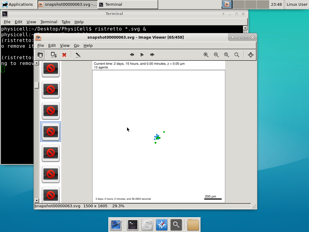 As a nice tip, you can press the left and right arrows to advance through the SVG images, or hold the right arrow down to advance through quickly.
Now, let’s use ImageMagick to convert the SVG files into JPG file: call “magick mogrify -format jpg snap*.svg”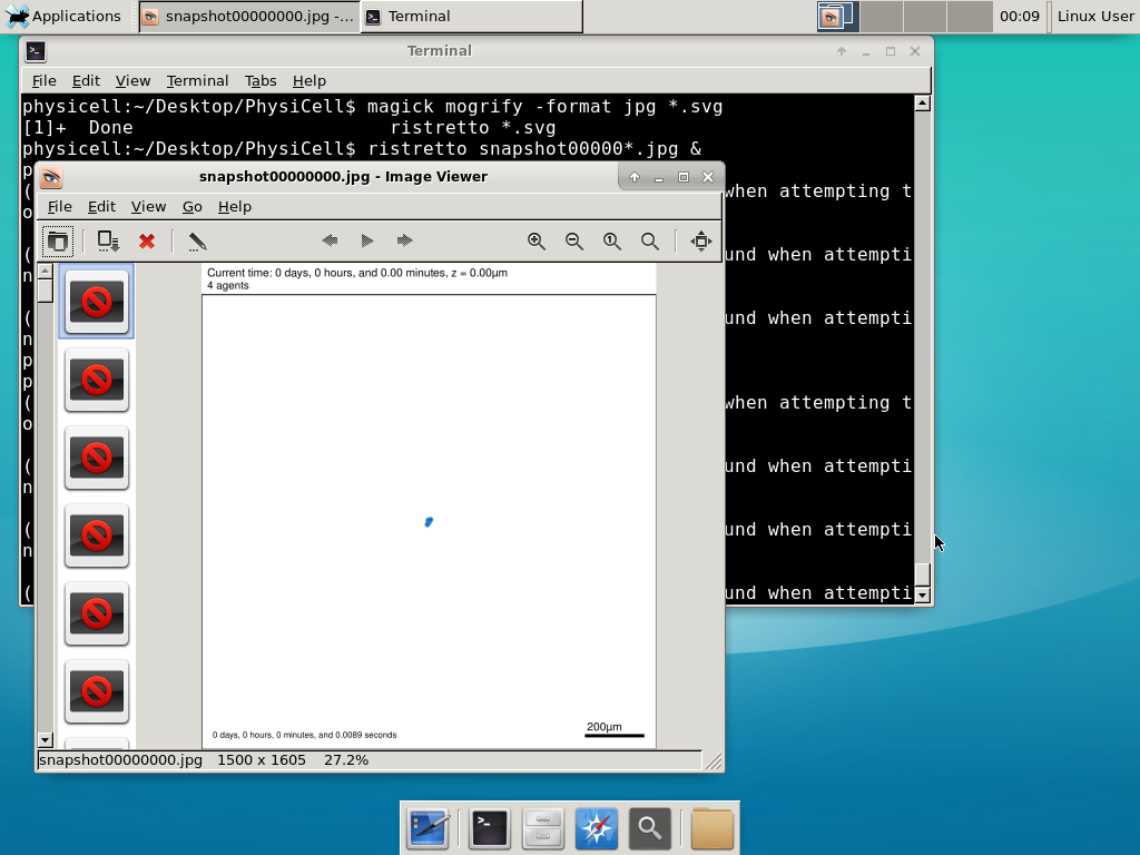
Next, let’s turn those images into a movie. I generally create moves that are 24 frames pers se, so that 1 second of the movie is 1 hour of simulations time. We’ll use mencoder, with options below given to help get a good quality vs. size tradeoff: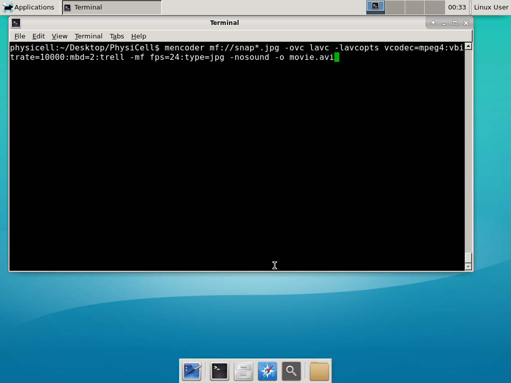
When you’re done, view the movie with mplayer. The options below scale the window to fit within the virtual monitor:
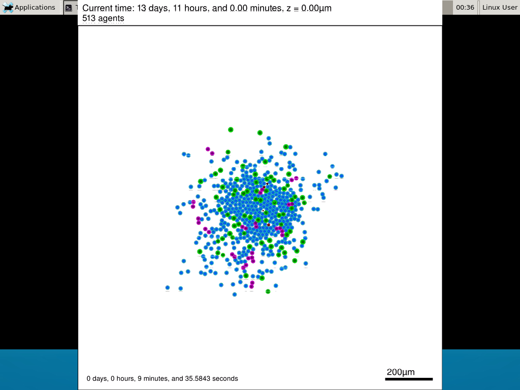
If you want to loop the movie, add “-loop 999” to your command.
7) Get familiar with other tools
Use nano (useage: nano <filename>) to quickly change files at the command line. Hit <control>-O to save your results. Hit <control>-X to exit. <control>-W will search within the file.
Use nedit (useage: nedit <filename> &) to open up one more text files in a graphical editor. This is a good way to edit multiple files at once.
Sometimes, you need to run commands at elevated (admin or root) privileges. Use sudo. Here’s an example, searching the Alpine Linux package manager apk for clang:
physicell:~$ sudo apk search gcc
[sudo] password for physicell:
physicell:~$ sudo apk search clang
clang-analyzer-4.0.0-r0
clang-libs-4.0.0-r0
clang-dev-4.0.0-r0
clang-static-4.0.0-r0
emscripten-fastcomp-1.37.10-r0
clang-doc-4.0.0-r0
clang-4.0.0-r0
physicell:~/Desktop/PhysiCell$
If you want to install clang/llvm (as an alternative compiler):
physicell:~$ sudo apk add gcc
[sudo] password for physicell:
physicell:~$ sudo apk search clang
clang-analyzer-4.0.0-r0
clang-libs-4.0.0-r0
clang-dev-4.0.0-r0
clang-static-4.0.0-r0
emscripten-fastcomp-1.37.10-r0
clang-doc-4.0.0-r0
clang-4.0.0-r0
physicell:~/Desktop/PhysiCell$
Notice that it asks for a password: use the password for root (which is physicell).
8) [Optional] Configure a shared folder
Coming soon.
Why both with zipped source, then?
Given that we can get a whole development environment by just downloading and importing a virtual appliance, why
bother with all the setup of a native development environment, like this tutorial (Windows) or this tutorial (Mac)?
One word: performance. In my testing, I still have not found the performance running inside a
virtual machine to match compiling and running directly on your system. So, the Virtual Appliance is a great
option to get up and running quickly while trying things out, but I still recommend setting up natively with
one of the tutorials I linked in the preceding paragraphs.
What’s next?
In the coming weeks, we’ll post further tutorials on using PhysiCell. In the meantime, have a look at the
PhysiCell project website, and these links as well:
- BioFVM on MathCancer.org: http://BioFVM.MathCancer.org
- BioFVM on SourceForge: http://BioFVM.sf.net
- BioFVM Method Paper in BioInformatics: http://dx.doi.org/10.1093/bioinformatics/btv730
- PhysiCell on MathCancer.org: http://PhysiCell.MathCancer.org
- PhysiCell on Sourceforge: http://PhysiCell.sf.net
- PhysiCell Method Paper (preprint): https://doi.org/10.1101/088773
- PhysiCell tutorials: [click here]