Day: September 19, 2017
Working with PhysiCell MultiCellDS digital snapshots in Matlab

PhysiCell 1.2.1 and later saves data as a specialized MultiCellDS digital snapshot, which includes chemical substrate fields, mesh information, and a readout of the cells and their phenotypes at single simulation time point. This tutorial will help you learn to use the matlab processing files included with PhysiCell.
This tutorial assumes you know (1) how to work at the shell / command line of your operating system, and (2) basic plotting and other functions in Matlab.
Key elements of a PhysiCell digital snapshot
A PhysiCell digital snapshot (a customized form of the MultiCellDS digital simulation snapshot) includes the following elements saved as XML and MAT files:
- output12345678.xml : This is the “base” output file, in MultiCellDS format. It includes key metadata such as when the file was created, the software, microenvironment information, and custom data saved at the simulation time. The Matlab files read this base file to find other related files (listed next). Example: output00003696.xml
- initial_mesh0.mat : This is the computational mesh information for BioFVM at time 0.0. Because BioFVM and PhysiCell do not use moving meshes, we do not save this data at any subsequent time.
- output12345678_microenvironment0.mat : This saves each biochemical substrate in the microenvironment at the computational voxels defined in the mesh (see above). Example: output00003696_microenvironment0.mat
- output12345678_cells.mat : This saves very basic cellular information related to BioFVM, including cell positions, volumes, secretion rates, uptake rates, and secretion saturation densities. Example: output00003696_cells.mat
- output12345678_cells_physicell.mat : This saves extra PhysiCell data for each cell agent, including volume information, cell cycle status, motility information, cell death information, basic mechanics, and any user-defined custom data. Example: output00003696_cells_physicell.mat
These snapshots make extensive use of Matlab Level 4 .mat files, for fast, compact, and well-supported saving of array data. Note that even if you cannot ready MultiCellDS XML files, you can work to parse the .mat files themselves.
The PhysiCell Matlab .m files
Every PhysiCell distribution includes some matlab functions to work with PhysiCell digital simulation snapshots, stored in the matlab subdirectory. The main ones are:
- composite_cutaway_plot.m : provides a quick, coarse 3-D cutaway plot of the discrete cells, with different colors for live (red), apoptotic (b), and necrotic (black) cells.
- read_MultiCellDS_xml.m : reads the “base” PhysiCell snapshot and its associated matlab files.
- set_MCDS_constants.m : creates a data structure MCDS_constants that has the same constants as PhysiCell_constants.h. This is useful for identifying cell cycle phases, etc.
- simple_cutaway_plot.m : provides a quick, coarse 3-D cutaway plot of user-specified cells.
- simple_plot.m : provides, a quick, coarse 3-D plot of the user-specified cells, without a cutaway or cross-sectional clipping plane.
A note on GNU Octave
Unfortunately, GNU octave does not include XML file parsing without some significant user tinkering. And one you’re done, it is approximately one order of magnitude slower than Matlab. Octave users can directly import the .mat files described above, but without the helpful metadata in the XML file. We’ll provide more information on the structure of these MAT files in a future blog post. Moreover, we plan to provide python and other tools for users without access to Matlab.
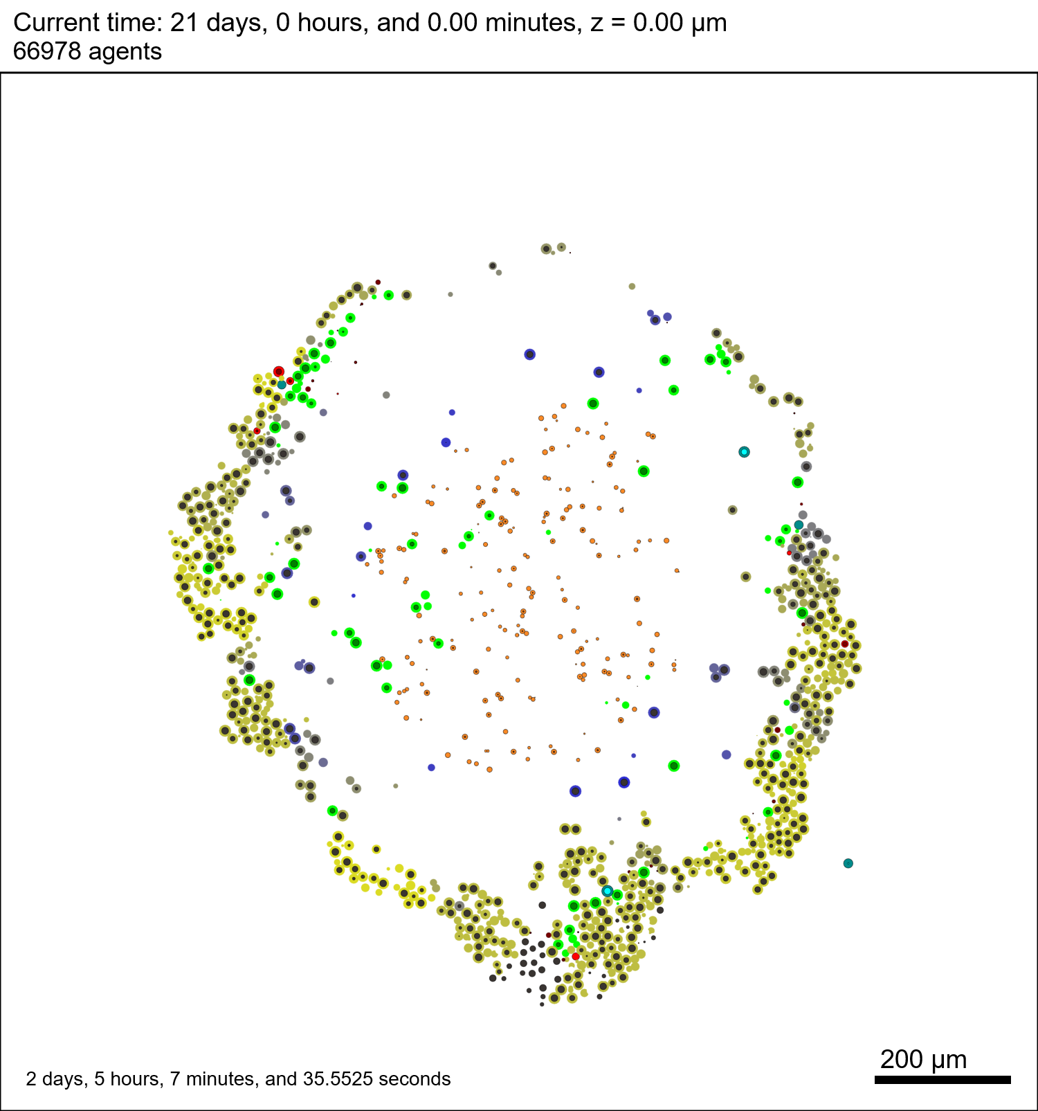
A sample digital snapshot
We provide a 3-D simulation snapshot from the final simulation time of the cancer-immune example in Ghaffarizadeh et al. (2017, in review) at:
The corresponding SVG cross-section for that time (through z = 0 μm) looks like this:
Unzip the sample dataset in any directory, and make sure the matlab files above are in the same directory (or in your Matlab path). If you’re inside matlab:
!unzip 3D_PhysiCell_matlab_sample.zip
Loading a PhysiCell MultiCellDS digital snapshot
Now, load the snapshot:
MCDS = read_MultiCellDS_xml( 'output00003696.xml');
This will load the mesh, substrates, and discrete cells into the MCDS data structure, and give a basic summary:
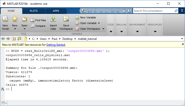
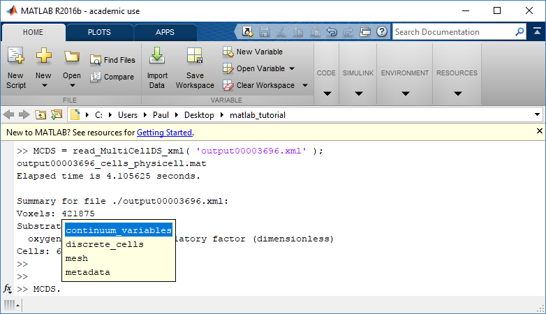
Typing ‘MCDS’ and then hitting ‘tab’ (for auto-completion) shows the overall structure of MCDS, stored as metadata, mesh, continuum variables, and discrete cells:
To get simulation metadata, such as the current simulation time, look at MCDS.metadata.current_time
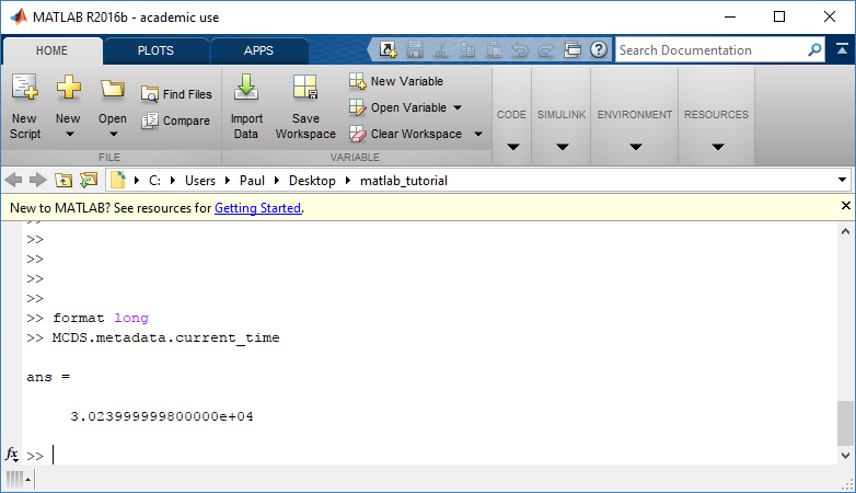
Here, we see that the current simulation time is 30240 minutes, or 21 days. MCDS.metadata.current_runtime gives the elapsed walltime to up to this point: about 53 hours (1.9e5 seconds), including file I/O time to write full simulation data once per 3 simulated minutes after the start of the adaptive immune response.
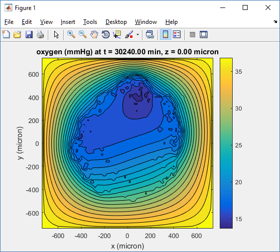
Plotting chemical substrates
Let’s make an oxygen contour plot through z = 0 μm. First, we find the index corresponding to this z-value:
k = find( MCDS.mesh.Z_coordinates == 0 );
Next, let’s figure out which variable is oxygen. Type “MCDS.continuum_variables.name”, which will show the array of variable names:
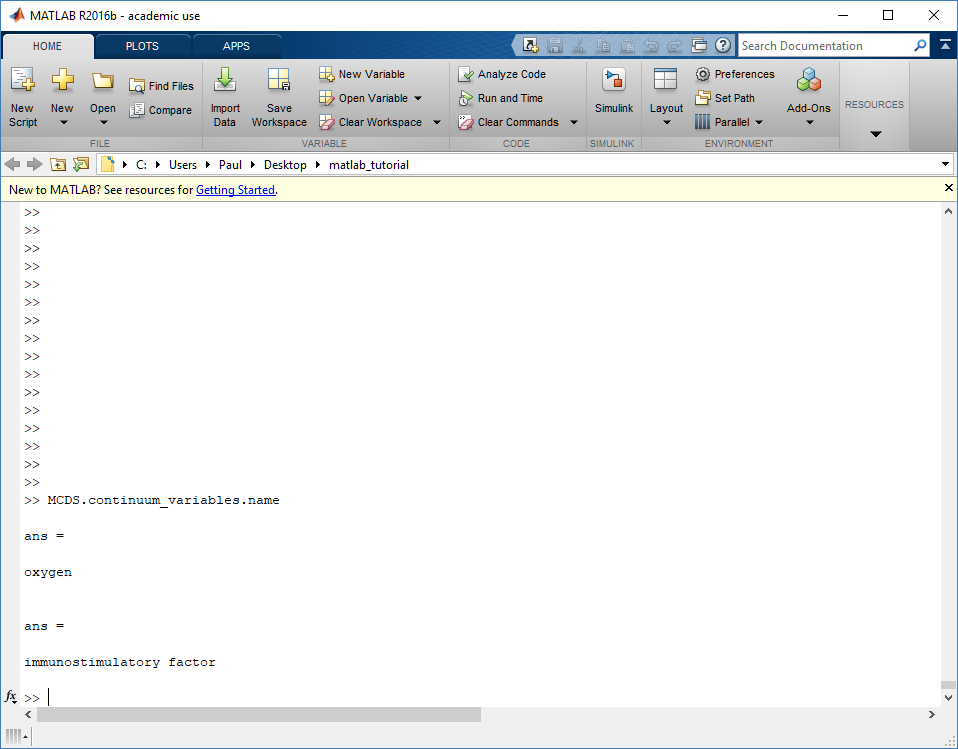
Here, oxygen is the first variable, (index 1). So, to make a filled contour plot:
contourf( MCDS.mesh.X(:,:,k), MCDS.mesh.Y(:,:,k), ...
     MCDS.continuum_variables(1).data(:,:,k) , 20 ) ;
Now, let’s set this to a correct aspect ratio (no stretching in x or y), add a colorbar, and set the axis labels, using
metadata to get labels:
axis image
colorbar
xlabel( sprintf( 'x (%s)' , MCDS.metadata.spatial_units) );
ylabel( sprintf( 'y (%s)' , MCDS.metadata.spatial_units) );
Lastly, let’s add an appropriate (time-based) title:
title( sprintf('%s (%s) at t = %3.2f %s, z = %3.2f %s', MCDS.continuum_variables(1).name , ...
     MCDS.continuum_variables(1).units , ...
     MCDS.metadata.current_time , ...
     MCDS.metadata.time_units, ...
     MCDS.mesh.Z_coordinates(k), ...
     MCDS.metadata.spatial_units ) );
Here’s the end result:
We can easily export graphics, such as to PNG format:
print( '-dpng' , 'output_o2.png' );
For more on plotting BioFVM data, see the tutorial
at http://www.mathcancer.org/blog/saving-multicellds-data-from-biofvm/
Plotting cells in space
3-D point cloud
First, let’s plot all the cells in 3D:
plot3( MCDS.discrete_cells.state.position(:,1) , MCDS.discrete_cells.state.position(:,2), ...
	MCDS.discrete_cells.state.position(:,3) , 'bo' );
At first glance, this does not look good: some cells are far out of the simulation domain, distorting the automatic range of the plot:
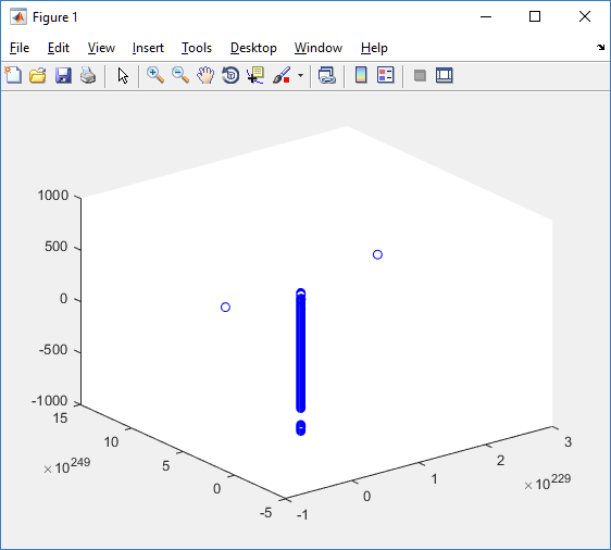
This does not ordinarily happen in PhysiCell (the default cell mechanics functions have checks to prevent such behavior), but this example includes a simple Hookean elastic adhesion model for immune cell attachment to tumor cells. In rare circumstances, an attached tumor cell or immune cell can apoptose on its own (due to its background apoptosis rate),
without “knowing” to detach itself from the surviving cell in the pair. The remaining cell attempts to calculate its elastic velocity based upon an invalid cell position (no longer in memory), creating an artificially large velocity that “flings” it out of the simulation domain. Such cells are not simulated any further, so this is effectively equivalent to an extra apoptosis event (only 3 cells are out of the simulation domain after tens of millions of cell-cell elastic adhesion calculations). Future versions of this example will include extra checks to prevent this rare behavior.
The plot can simply be fixed by changing the axis:
axis( 1000*[-1 1 -1 1 -1 1] )
axis square
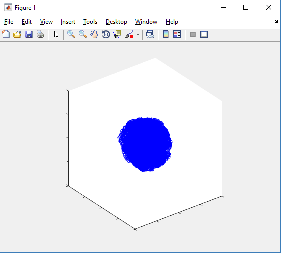
Notice that this is a very difficult plot to read, and very non-interactive (laggy) to rotation and scaling operations. We can make a slightly nicer plot by searching for different cell types and plotting them with different colors:
% make it easier to work with the cell positions;
P = MCDS.discrete_cells.state.position;

% find type 1 cells
ind1 = find( MCDS.discrete_cells.metadata.type == 1 );
% better still, eliminate those out of the simulation domain
ind1 = find( MCDS.discrete_cells.metadata.type == 1 & ...
    abs(P(:,1))' < 1000 & abs(P(:,2))' < 1000 & abs(P(:,3))' < 1000 );

% find type 0 cells
ind0 = find( MCDS.discrete_cells.metadata.type == 0 & ...
    abs(P(:,1))' < 1000 & abs(P(:,2))' < 1000 & abs(P(:,3))' < 1000 );

%now plot them
P = MCDS.discrete_cells.state.position;
plot3( P(ind0,1), P(ind0,2), P(ind0,3), 'bo' )
hold on
plot3( P(ind1,1), P(ind1,2), P(ind1,3), 'ro' )
hold off
axis( 1000*[-1 1 -1 1 -1 1] )
axis square
However, this isn’t much better. You can use the scatter3 function to gain more control on the size and color of the plotted cells, or even make macros to plot spheres in the cell locations (with shading and lighting), but Matlab is very slow when plotting beyond 103 cells. Instead, we recommend the faster preview functions below for data exploration, and higher-quality plotting (e.g., by POV-ray) for final publication-
Fast 3-D cell data previewers
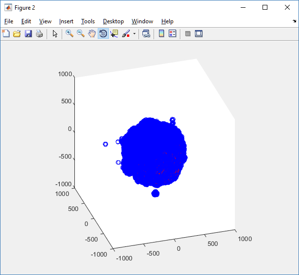
Notice that plot3 and scatter3 are painfully slow for any nontrivial number of cells. We can use a few fast previewers to quickly get a sense of the data. First, let’s plot all the dead cells, and make them red:
clf
simple_plot( MCDS,  MCDS, MCDS.discrete_cells.dead_cells , 'r' )
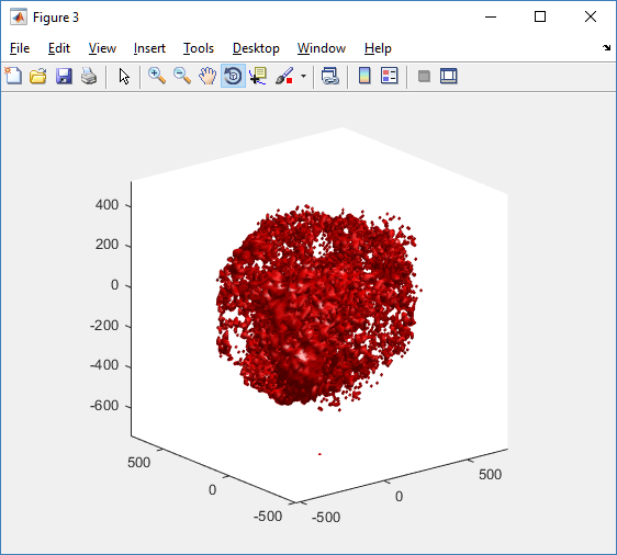
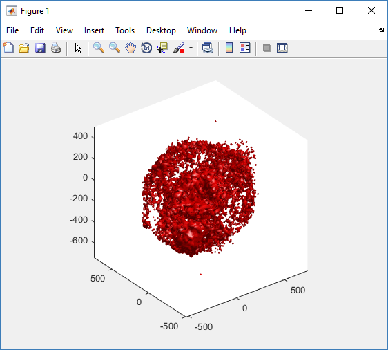
This function creates a coarse-grained 3-D indicator function (0 if no cells are present; 1 if they are), and plots a 3-D level surface. It is very responsive to rotations and other operations to explore the data. You may notice the second argument is a list of indices: only these cells are plotted. This gives you a method to select cells with specific characteristics when plotting. (More on that below.) If you want to get a sense of the interior structure, use a cutaway plot:
clf
simple_cutaway_plot( MCDS, MCDS, MCDS.discrete_cells.dead_cells , 'r' )
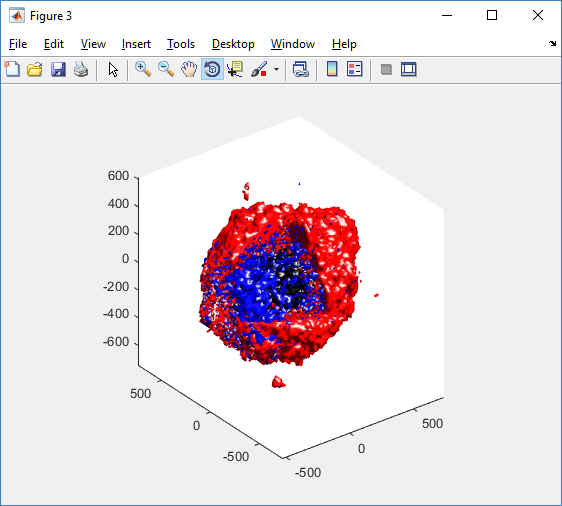
We also provide a fast “composite” cutaway which plots all live cells as red, apoptotic cells as blue (without the cutaway), and all necrotic cells as black:
clf
composite_cutaway_plot( MCDS )
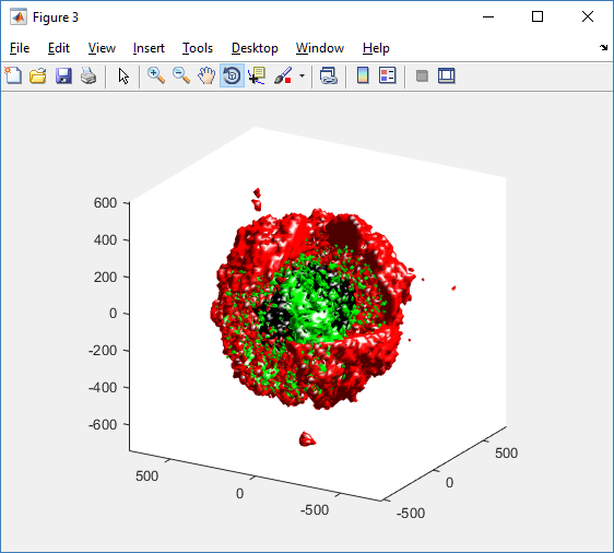
Lastly, we show an improved plot that uses different colors for the immune cells, and Matlab’s “find” function to help set up the indexing:
constants = set_MCDS_constants

% find the type 0 necrotic cells
ind0_necrotic = find( MCDS.discrete_cells.metadata.type == 0 & ...
    (MCDS.discrete_cells.phenotype.cycle.current_phase == constants.necrotic_swelling | ...
    MCDS.discrete_cells.phenotype.cycle.current_phase == constants.necrotic_lysed | ...
    MCDS.discrete_cells.phenotype.cycle.current_phase == constants.necrotic) );

% find the live type 0 cells
ind0_live = find( MCDS.discrete_cells.metadata.type == 0 & ...
    (MCDS.discrete_cells.phenotype.cycle.current_phase ~= constants.necrotic_swelling & ...
    MCDS.discrete_cells.phenotype.cycle.current_phase ~= constants.necrotic_lysed & ...
    MCDS.discrete_cells.phenotype.cycle.current_phase ~= constants.necrotic & ...
    MCDS.discrete_cells.phenotype.cycle.current_phase ~= constants.apoptotic) );

clf
% plot live tumor cells red, in cutaway view
simple_cutaway_plot( MCDS, ind0_live , 'r' );
hold on
% plot dead tumor cells black, in cutaway view
simple_cutaway_plot( MCDS, ind0_necrotic , 'k' )
% plot all immune cells, but without cutaway (to show how they infiltrate)
simple_plot( MCDS, ind1, 'g' )
hold off
A small cautionary note on future compatibility
PhysiCell 1.2.1 uses the <custom> data tag (allowed as part of the MultiCellDS specification) to encode its cell data, to allow a more compact data representation, because the current PhysiCell daft does not support such a formulation, and Matlab is painfully slow at parsing XML files larger than ~50 MB. Thus, PhysiCell snapshots are not yet fully compatible with general MultiCellDS tools, which would by default ignore custom data. In the future, we will make available converter utilities to transform “native” custom PhysiCell snapshots to MultiCellDS snapshots that encode all the cellular information in a more verbose but compatible XML format.
Closing words and future work
Because Octave is not a great option for parsing XML files (with critical MultiCellDS metadata), we plan to write similar functions to read and plot PhysiCell snapshots in Python, as an open source alternative. Moreover, our lab in the next year will focus on creating further MultiCellDS configuration, analysis, and visualization routines. We also plan to provide additional 3-D functions for plotting the discrete cells and varying color with their properties.
In the longer term, we will develop open source, stand-alone analysis and visualization tools for MultiCellDS snapshots (including PhysiCell snapshots). Please stay tuned!