Month: October 2019
PhysiCell Tools : python-loader
The newest tool for PhysiCell provides an easy way to load your PhysiCell output data into python for analysis. This builds upon previous work on loading data into MATLAB. A post on that tool can be found at:
http://www.mathcancer.org/blog/working-with-physicell-snapshots-in-matlab/.
PhysiCell stores output data as a MultiCell Digital Snapshot (MultiCellDS) that consists of several files for each time step and is probably stored in your ./output directory. pyMCDS is a python object that is initialized with the .xml file
What you’ll need
- python-loader, available on GitHub at
- Python 3.x, recommended distribution available at
- A number of Python packages, included in anaconda or available through pip
- NumPy
- pandas
- scipy
- Some PhysiCell data, probably in your ./output directory
Anatomy of a MultiCell Digital Snapshot
Each time PhysiCell’s internal time tracker passes a time step where data is to be saved, it generates a number of files of various types. Each of these files will have a number at the end that indicates where it belongs in the sequence of outputs. All of the files from the first round of output will end in 00000000.* and the second round will be 00000001.* and so on. Let’s say we’re interested in a set of output from partway through the run, the 88th set of output files. The files we care about most from this set consists of:
- output00000087.xml: This file is the main organizer of the data. It contains an overview of the data stored in the MultiCellDS as well as some actual data including:
- Metadata about the time and runtime for the current time step
- Coordinates for the computational domain
- Parameters for diffusing substrates in the microenvironment
- Column labels for the cell data
- File names for the files that contain microenvironment and cell data at this time step
- output00000087_microenvironment0.mat: This is a MATLAB matrix file that contains all of the data about the microenvironment at this time step
- output00000087_cells_physicell.mat: This is a MATLAB matrix file that contains all of the tracked information about the individual cells in the model. It tells us things like the cells’ position, volume, secretion, cell cycle status, and user-defined cell parameters.
Setup
Using pyMCDS
From the appropriate file in your PhysiCell directory, wherever pyMCDS.py lives, you can use the data loader in your own scripts or in an interactive session. To start you have to import the pyMCDS class
from pyMCDS import pyMCDS
Loading the data
Data is loaded into python from the MultiCellDS by initializing the pyMCDS object. The initialization function for pyMCDS takes one required and one optional argument.
__init__(xml_file, [output_path = '.'])
    '''
    xml_file : string
        String containing the name of the output xml file
    output_path :
        String containing the path (relative or absolute) to the directory
        where PhysiCell output files are stored
    '''
We are interested in reading output00000087.xml that lives in ~/path/to/PhysiCell/output (don’t worry Windows paths work too). We would initialize our pyMCDS object using those names and the actual data would be stored in a member dictionary called data.
mcds = pyMCDS('output00000087.xml', '~/path/to/PhysiCell/output')
# Now our data lives in:
mcds.data
We’ve tried to keep everything organized inside of this dictionary but let’s take a look at what we actually have in here. Of course in real output, there will probably not be a chemical named my_chemical, this is simply there to illustrate how multiple chemicals are handled.

The data member dictionary is a dictionary of dictionaries whose child dictionaries can be accessed through normal python dictionary syntax.
mcds.data['metadata']
mcds.data['continuum_variables']['my_chemical']
Each of these subdictionaries contains data, we will take a look at exactly what that data is and how it can be accessed in the following sections.
Metadata
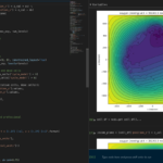
The metadata dictionary contains information about the time of the simulation as well as units for both times and space. Here and in later sections blue boxes indicate scalars and green boxes indicate strings. We can access each of these things using normal dictionary syntax. We’ve also got access to a helper function get_time() for the common operation of retrieving the simulation time.
>>> mcds.data['metadata']['time_units']
'min'
>>> mcds.get_time()
5220.0
Mesh
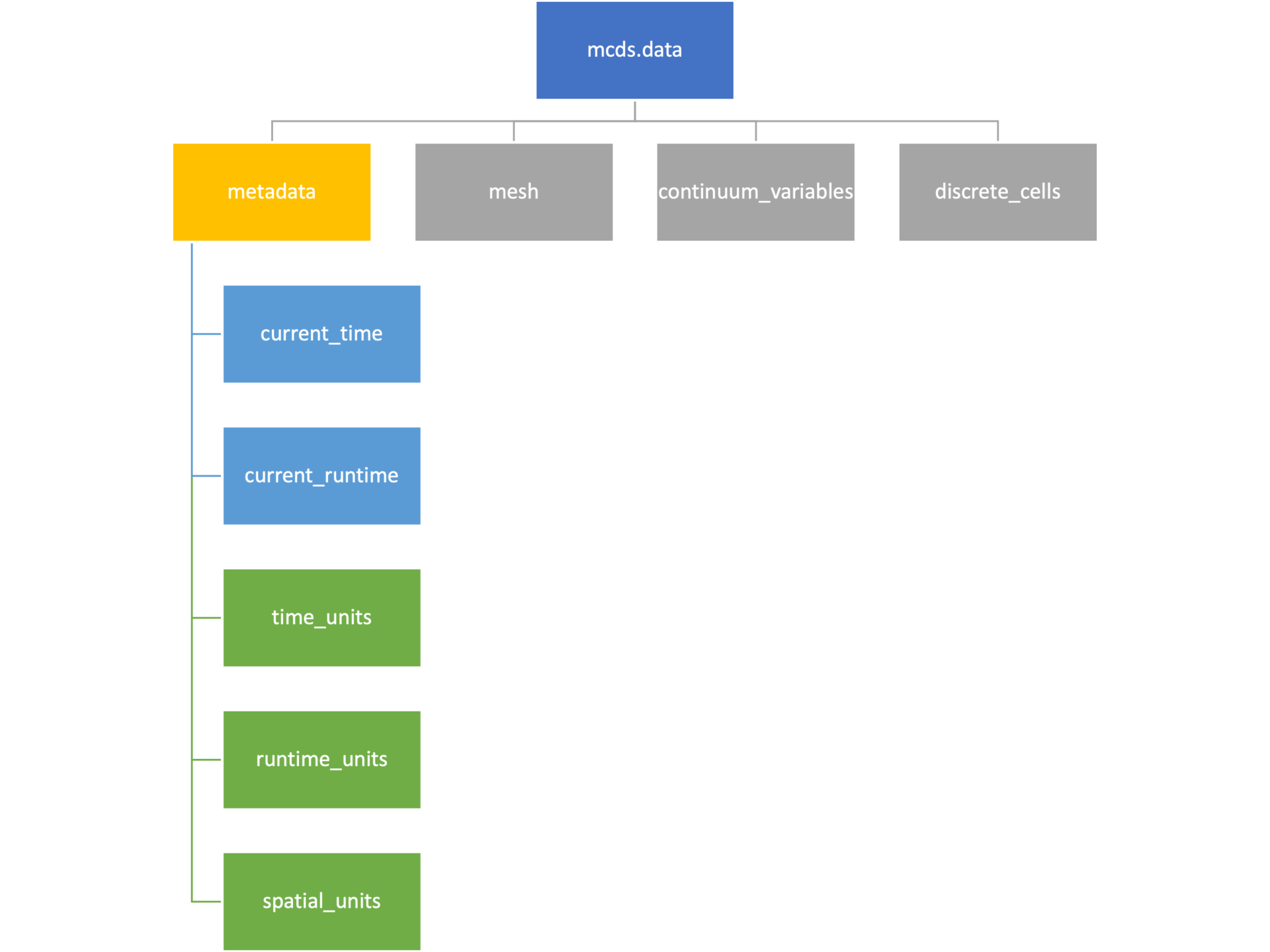
The mesh dictionary has a lot more going on than the metadata dictionary. It contains three numpy arrays, indicated by orange boxes, as well as another dictionary. The three arrays contain \(x\), \(y\) and \(z\) coordinates for the centers of the voxels that constiture the computational domain in a meshgrid format. This means that each of those arrays is tensors of rank three. Together they identify the coordinates of each possible point in the space.
In contrast, the arrays in the voxel dictionary are stored linearly. If we know that we care about voxel number 42, we want to use the stuff in the voxels dictionary. If we want to make a contour plot, we want to use the x_coordinates, y_coordinates, and z_coordinates arrays.
# We can extract one of the meshgrid arrays as a numpy array
>>> y_coords = mcds.data['mesh']['y_coordinates']
>>> y_coords.shape
(75, 75, 75)
>>> y_coords[0, 0, :4]
array([-740., -740., -740., -740.])

# We can also extract the array of voxel centers
>>> centers = mcds.data['mesh']['voxels']['centers']
>>> centers.shape
(3, 421875)
>>> centers[:, :4]
array([[-740., -720., -700., -680.],
       [-740., -740., -740., -740.],
       [-740., -740., -740., -740.]])

# We have a handy function to quickly extract the components of the full meshgrid
>>> xx, yy, zz = mcds.get_mesh()
>>> yy.shape
(75, 75, 75)
>>> yy[0, 0, :4]
array([-740., -740., -740., -740.])

# We can also use this to return the meshgrid describing an x, y plane
>>> xx, yy = mcds.get_2D_mesh()
>>> yy.shape
(75, 75)
Continuum variables
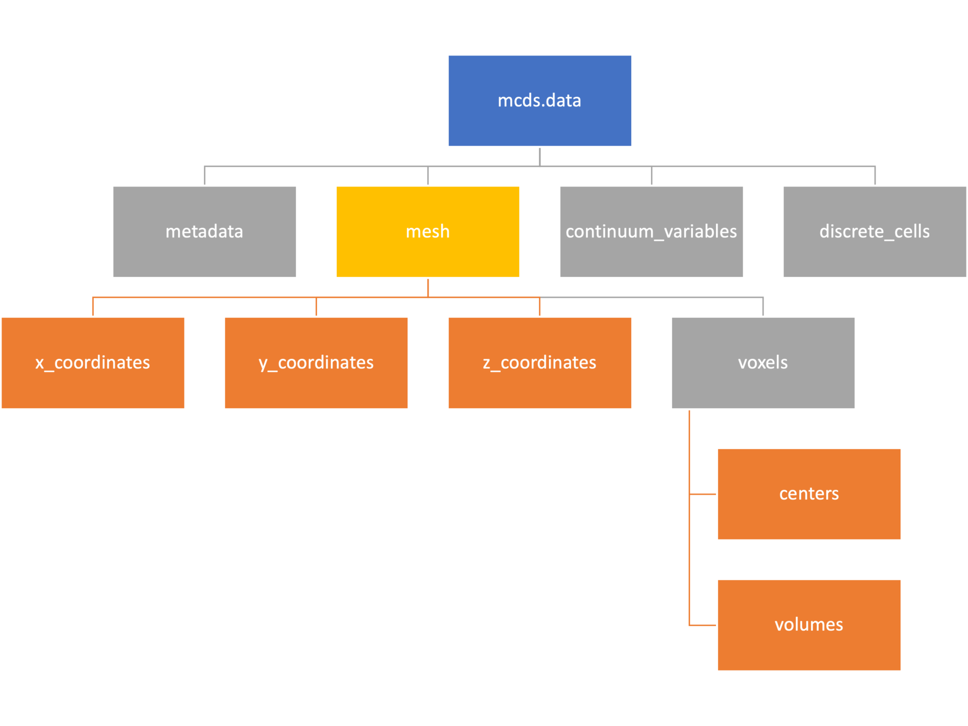
The continuum_variables dictionary is the most complicated of the four. It contains subdictionaries that we access using the names of each of the chemicals in the microenvironment. In our toy example above, these are oxygen and my_chemical. If our model tracked diffusing oxygen, VEGF, and glucose, then the continuum_variables dictionary would contain a subdirectory for each of them.
For a particular chemical species in the microenvironment we have two more dictionaries called decay_rate and diffusion_coefficient, and a numpy array called data. The diffusion and decay dictionaries each complete the value stored as a scalar and the unit stored as a string. The numpy array contains the concentrations of the chemical in each voxel at this time and is the same shape as the meshgrids of the computational domain stored in the .data[‘mesh’] arrays.
# we need to know the names of the substrates to work with
# this data. We have a function to help us find them.
>>> mcds.get_substrate_names()
['oxygen', 'my_chemical']

# The diffusable chemical dictionaries are messy
# if we need to do a lot with them it might be easier
# to put them into their own instance
>>> oxy_dict = mcds.data['continuum_variables']['oxygen']
>>> oxy_dict['decay_rate']
{'value': 0.1, 'units': '1/min'}

# What we care about most is probably the numpy
# array of concentrations
>>> oxy_conc = oxy_dict['data']
>>> oxy_conc.shape
(75, 75, 75)

# Alternatively, we can get the same array with a function
>>> oxy_conc2 = mcds.get_concentrations('oxygen')
>>> oxy_conc2.shape
(75, 75, 75)

# We can also get the concentrations on a plane using the
# same function and supplying a z value to "slice through"
# note that right now the z_value must be an exact match
# for a plane of voxel centers, in the future we may add
# interpolation.
>>> oxy_plane = mcds.get_concentrations('oxygen', z_value=100.0)
>>> oxy_plane.shape
(75, 75)

# we can also find the concentration in a single voxel using the
# position of a point within that voxel. This will give us an
# array of all concentrations at that point.
>>> mcds.get_concentrations_at(x=0., y=550., z=0.)
array([17.94514446,  0.99113448])
Discrete Cells

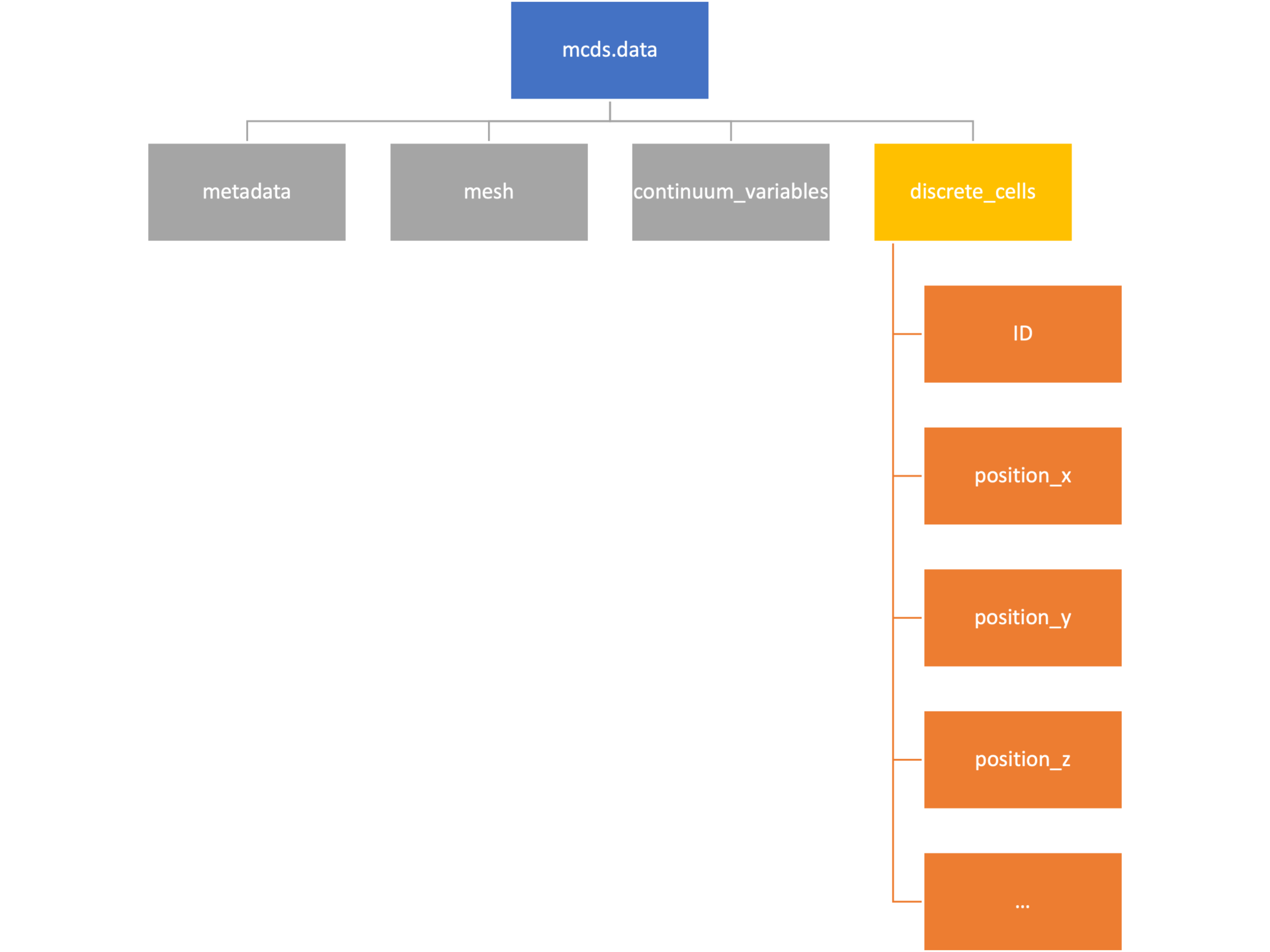
The discrete cells dictionary is relatively straightforward. It contains a number of numpy arrays that contain information regarding individual cells. These are all 1-dimensional arrays and each corresponds to one of the variables specified in the output*.xml file. With the default settings, these are:
- ID: unique integer that will identify the cell throughout its lifetime in the simulation
- position(_x, _y, _z): floating point positions for the cell in \(x\), \(y\), and \(z\) directions
- total_volume: total volume of the cell
- cell_type: integer label for the cell as used in PhysiCell
- cycle_model: integer label for the cell cycle model as used in PhysiCell
- current_phase: integer specification for which phase of the cycle model the cell is currently in
- elapsed_time_in_phase: time that cell has been in current phase of cell cycle model
- nuclear_volume: volume of cell nucleus
- cytoplasmic_volume: volume of cell cytoplasm
- fluid_fraction: proportion of the volume due to fliud
- calcified_fraction: proportion of volume consisting of calcified material
- orientation(_x, _y, _z): direction in which cell is pointing
- polarity:
- migration_speed: current speed of cell
- motility_vector(_x, _y, _z): current direction of movement of cell
- migration_bias: coefficient for stochastic movement (higher is “more deterministic”)
- motility_bias_direction(_x, _y, _z): direction of movement bias
- persistence_time: time in-between direction changes for cell
- motility_reserved:
# Extracting single variables is just like before
>>> cell_ids = mcds.data['discrete_cells']['ID']
>>> cell_ids.shape
(18595,)
>>> cell_ids[:4]
array([0., 1., 2., 3.])

# If we're clever we can extract 2D arrays
>>> cell_vec = np.zeros((cell_ids.shape[0], 3))
>>> vec_list = ['position_x', 'position_y', 'position_z']
>>> for i, lab in enumerate(vec_list):
...     cell_vec[:, i] = mcds.data['discrete_cells'][lab]
...
array([[ -69.72657128,  -39.02046405, -233.63178904],
       [ -69.84507464,  -22.71693265, -233.59277388],
       [ -69.84891462,   -6.04070516, -233.61816711],
       [ -69.845265  ,   10.80035554, -233.61667313]])

# We can get the list of all of the variables stored in this dictionary
>>> mcds.get_cell_variables()
['ID',
 'position_x',
 'position_y',
 'position_z',
 'total_volume',
 'cell_type',
 'cycle_model',
 'current_phase',
 'elapsed_time_in_phase',
 'nuclear_volume',
 'cytoplasmic_volume',
 'fluid_fraction',
 'calcified_fraction',
 'orientation_x',
 'orientation_y',
 'orientation_z',
 'polarity',
 'migration_speed',
 'motility_vector_x',
 'motility_vector_y',
 'motility_vector_z',
 'migration_bias',
 'motility_bias_direction_x',
 'motility_bias_direction_y',
 'motility_bias_direction_z',
 'persistence_time',
 'motility_reserved',
 'oncoprotein',
 'elastic_coefficient',
 'kill_rate',
 'attachment_lifetime',
 'attachment_rate']
# We can also get all of the cell data as a pandas DataFrame
>>> cell_df = mcds.get_cell_df()
>>> cell_df.head()
ID     position_x   position_y    position_z total_volume cell_type cycle_model ...
0.0   - 69.726571  - 39.020464  - 233.631789       2494.0       0.0         5.0 ...
1.0   - 69.845075  - 22.716933  - 233.592774       2494.0       0.0         5.0 ...
2.0   - 69.848915  - 6.040705   - 233.618167       2494.0       0.0         5.0 ...
3.0   - 69.845265    10.800356  - 233.616673       2494.0       0.0         5.0 ...
4.0   - 69.828161    27.324530  - 233.631579       2494.0       0.0         5.0 ...

# if we want to we can also get just the subset of cells that
# are in a specific voxel
>>> vox_df = mcds.get_cell_df_at(x=0.0, y=550.0, z=0.0)
>>> vox_df.iloc[:, :5]
             ID  position_x  position_y  position_z  total_volume
26718  228761.0    6.623617  536.709341   -1.282934   2454.814507
52736  270274.0   -7.990034  538.184921    9.648955   1523.386488
Examples
These examples will not be made using our toy dataset described above but will instead be made using a single timepoint dataset that can be found at:
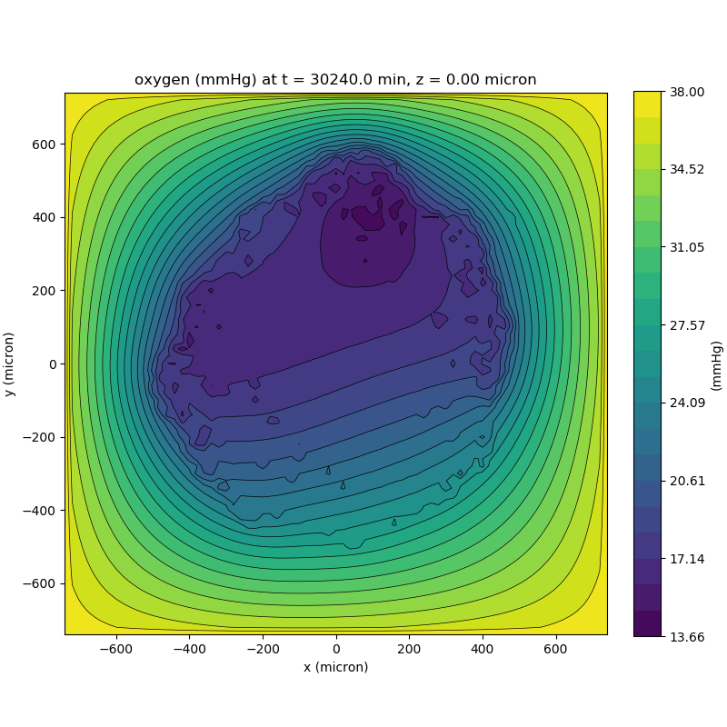
Substrate contour plot
One of the big advantages of working with PhysiCell data in python is that we have access to its plotting tools. For the sake of example let’s plot the partial pressure of oxygen throughout the computational domain along the \(z = 0\) plane. Once we’ve loaded our data by initializing a pyMCDS object, we can work entirely within python to produce the plot.
from pyMCDS import pyMCDS
import numpy as np
import matplotlib.pyplot as plt

# load data
mcds = pyMCDS('output00003696.xml', '../output')

# Set our z plane and get our substrate values along it
z_val = 0.00
plane_oxy = mcds.get_concentrations('oxygen', z_slice=z_val)

# Get the 2D mesh for contour plotting
xx, yy = mcds.get_mesh()

# We want to be able to control the number of contour levels so we
# need to do a little set up
num_levels = 21
min_conc = plane_oxy.min()
max_conc = plane_oxy.max()
my_levels = np.linspace(min_conc, max_conc, num_levels)

# set up the figure area and add data layers
fig, ax = plt.subplot()
cs = ax.contourf(xx, yy, plane_oxy, levels=my_levels)
ax.contour(xx, yy, plane_oxy, color='black', levels = my_levels,
           linewidths=0.5)

# Now we need to add our color bar
cbar1 = fig.colorbar(cs, shrink=0.75)
cbar1.set_label('mmHg')

# Let's put the time in to make these look nice
ax.set_aspect('equal')
ax.set_xlabel('x (micron)')
ax.set_ylabel('y (micron)')
ax.set_title('oxygen (mmHg) at t = {:.1f} {:s}, z = {:.2f} {:s}'.format(
                                        mcds.get_time(),
                                        mcds.data['metadata']['time_units'],
                                        z_val,
                                        mcds.data['metadata']['spatial_units'])

plt.show()
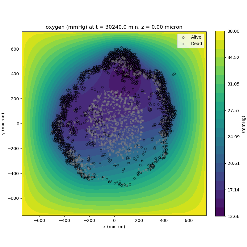
Adding a cells layer
We can also use pandas to do fairly complex selections of cells to add to our plots. Below we use pandas and the previous plot to add a cells layer.
from pyMCDS import pyMCDS
import numpy as np
import matplotlib.pyplot as plt

# load data
mcds = pyMCDS('output00003696.xml', '../output')

# Set our z plane and get our substrate values along it
z_val = 0.00
plane_oxy = mcds.get_concentrations('oxygen', z_slice=z_val)

# Get the 2D mesh for contour plotting
xx, yy = mcds.get_mesh()

# We want to be able to control the number of contour levels so we
# need to do a little set up
num_levels = 21
min_conc = plane_oxy.min()
max_conc = plane_oxy.max()
my_levels = np.linspace(min_conc, max_conc, num_levels)

# get our cells data and figure out which cells are in the plane
cell_df = mcds.get_cell_df()
ds = mcds.get_mesh_spacing()
inside_plane = (cell_df['position_z'] < z_val + ds) \ & (cell_df['position_z'] > z_val - ds)
plane_cells = cell_df[inside_plane]

# We're going to plot two types of cells and we want it to look nice
colors = ['black', 'grey']
sizes = [20, 8]
labels = ['Alive', 'Dead']

# set up the figure area and add microenvironment layer
fig, ax = plt.subplot()
cs = ax.contourf(xx, yy, plane_oxy, levels=my_levels)

# get our cells of interest
# alive_cells = plane_cells[plane_cells['cycle_model'] < 6]
# dead_cells = plane_cells[plane_cells['cycle_model'] > 6]
# -- for newer versions of PhysiCell
alive_cells = plane_cells[plane_cells['cycle_model'] < 100]
dead_cells = plane_cells[plane_cells['cycle_model'] >= 100]

# plot the cell layer
for i, plot_cells in enumerate((alive_cells, dead_cells)):
    ax.scatter(plot_cells['position_x'].values,
            plot_cells['position_y'].values,
            facecolor='none',
            edgecolors=colors[i],
            alpha=0.6,
            s=sizes[i],
            label=labels[i])

# Now we need to add our color bar
cbar1 = fig.colorbar(cs, shrink=0.75)
cbar1.set_label('mmHg')

# Let's put the time in to make these look nice
ax.set_aspect('equal')
ax.set_xlabel('x (micron)')
ax.set_ylabel('y (micron)')
ax.set_title('oxygen (mmHg) at t = {:.1f} {:s}, z = {:.2f} {:s}'.format(
                                        mcds.get_time(),
                                        mcds.data['metadata']['time_units'],
                                        z_val,
                                        mcds.data['metadata']['spatial_units'])
ax.legend(loc='upper right')

plt.show()
Future Direction
The first extension of this project will be timeseries functionality. This will provide similar data loading functionality but for a time series of MultiCell Digital Snapshots instead of simply one point in time.