Category: MathCancer
PhysiCell Tools : python-loader
The newest tool for PhysiCell provides an easy way to load your PhysiCell output data into python for analysis. This builds upon previous work on loading data into MATLAB. A post on that tool can be found at:
http://www.mathcancer.org/blog/working-with-physicell-snapshots-in-matlab/.
PhysiCell stores output data as a MultiCell Digital Snapshot (MultiCellDS) that consists of several files for each time step and is probably stored in your ./output directory. pyMCDS is a python object that is initialized with the .xml file
What you’ll need
- python-loader, available on GitHub at
- Python 3.x, recommended distribution available at
- A number of Python packages, included in anaconda or available through pip
- NumPy
- pandas
- scipy
- Some PhysiCell data, probably in your ./output directory
Anatomy of a MultiCell Digital Snapshot
Each time PhysiCell’s internal time tracker passes a time step where data is to be saved, it generates a number of files of various types. Each of these files will have a number at the end that indicates where it belongs in the sequence of outputs. All of the files from the first round of output will end in 00000000.* and the second round will be 00000001.* and so on. Let’s say we’re interested in a set of output from partway through the run, the 88th set of output files. The files we care about most from this set consists of:
- output00000087.xml: This file is the main organizer of the data. It contains an overview of the data stored in the MultiCellDS as well as some actual data including:
- Metadata about the time and runtime for the current time step
- Coordinates for the computational domain
- Parameters for diffusing substrates in the microenvironment
- Column labels for the cell data
- File names for the files that contain microenvironment and cell data at this time step
- output00000087_microenvironment0.mat: This is a MATLAB matrix file that contains all of the data about the microenvironment at this time step
- output00000087_cells_physicell.mat: This is a MATLAB matrix file that contains all of the tracked information about the individual cells in the model. It tells us things like the cells’ position, volume, secretion, cell cycle status, and user-defined cell parameters.
Setup
Using pyMCDS
From the appropriate file in your PhysiCell directory, wherever pyMCDS.py lives, you can use the data loader in your own scripts or in an interactive session. To start you have to import the pyMCDS class
from pyMCDS import pyMCDS
Loading the data
Data is loaded into python from the MultiCellDS by initializing the pyMCDS object. The initialization function for pyMCDS takes one required and one optional argument.
__init__(xml_file, [output_path = '.'])
    '''
    xml_file : string
        String containing the name of the output xml file
    output_path :
        String containing the path (relative or absolute) to the directory
        where PhysiCell output files are stored
    '''
We are interested in reading output00000087.xml that lives in ~/path/to/PhysiCell/output (don’t worry Windows paths work too). We would initialize our pyMCDS object using those names and the actual data would be stored in a member dictionary called data.
mcds = pyMCDS('output00000087.xml', '~/path/to/PhysiCell/output')
# Now our data lives in:
mcds.data
We’ve tried to keep everything organized inside of this dictionary but let’s take a look at what we actually have in here. Of course in real output, there will probably not be a chemical named my_chemical, this is simply there to illustrate how multiple chemicals are handled.

The data member dictionary is a dictionary of dictionaries whose child dictionaries can be accessed through normal python dictionary syntax.
mcds.data['metadata']
mcds.data['continuum_variables']['my_chemical']
Each of these subdictionaries contains data, we will take a look at exactly what that data is and how it can be accessed in the following sections.
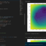
Metadata
The metadata dictionary contains information about the time of the simulation as well as units for both times and space. Here and in later sections blue boxes indicate scalars and green boxes indicate strings. We can access each of these things using normal dictionary syntax. We’ve also got access to a helper function get_time() for the common operation of retrieving the simulation time.
>>> mcds.data['metadata']['time_units']
'min'
>>> mcds.get_time()
5220.0
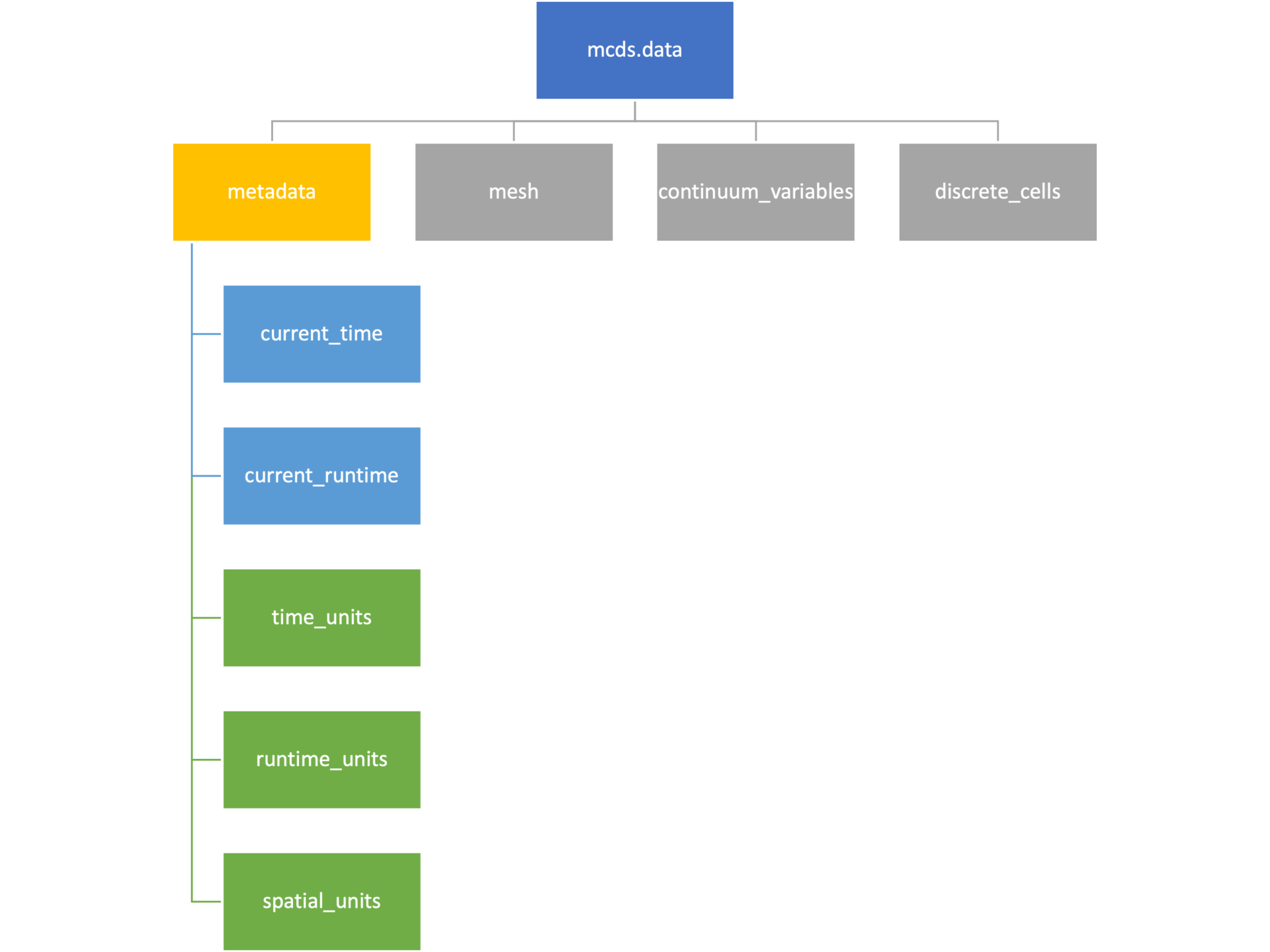
Mesh
The mesh dictionary has a lot more going on than the metadata dictionary. It contains three numpy arrays, indicated by orange boxes, as well as another dictionary. The three arrays contain \(x\), \(y\) and \(z\) coordinates for the centers of the voxels that constiture the computational domain in a meshgrid format. This means that each of those arrays is tensors of rank three. Together they identify the coordinates of each possible point in the space.
In contrast, the arrays in the voxel dictionary are stored linearly. If we know that we care about voxel number 42, we want to use the stuff in the voxels dictionary. If we want to make a contour plot, we want to use the x_coordinates, y_coordinates, and z_coordinates arrays.
# We can extract one of the meshgrid arrays as a numpy array
>>> y_coords = mcds.data['mesh']['y_coordinates']
>>> y_coords.shape
(75, 75, 75)
>>> y_coords[0, 0, :4]
array([-740., -740., -740., -740.])

# We can also extract the array of voxel centers
>>> centers = mcds.data['mesh']['voxels']['centers']
>>> centers.shape
(3, 421875)
>>> centers[:, :4]
array([[-740., -720., -700., -680.],
       [-740., -740., -740., -740.],
       [-740., -740., -740., -740.]])

# We have a handy function to quickly extract the components of the full meshgrid
>>> xx, yy, zz = mcds.get_mesh()
>>> yy.shape
(75, 75, 75)
>>> yy[0, 0, :4]
array([-740., -740., -740., -740.])

# We can also use this to return the meshgrid describing an x, y plane
>>> xx, yy = mcds.get_2D_mesh()
>>> yy.shape
(75, 75)
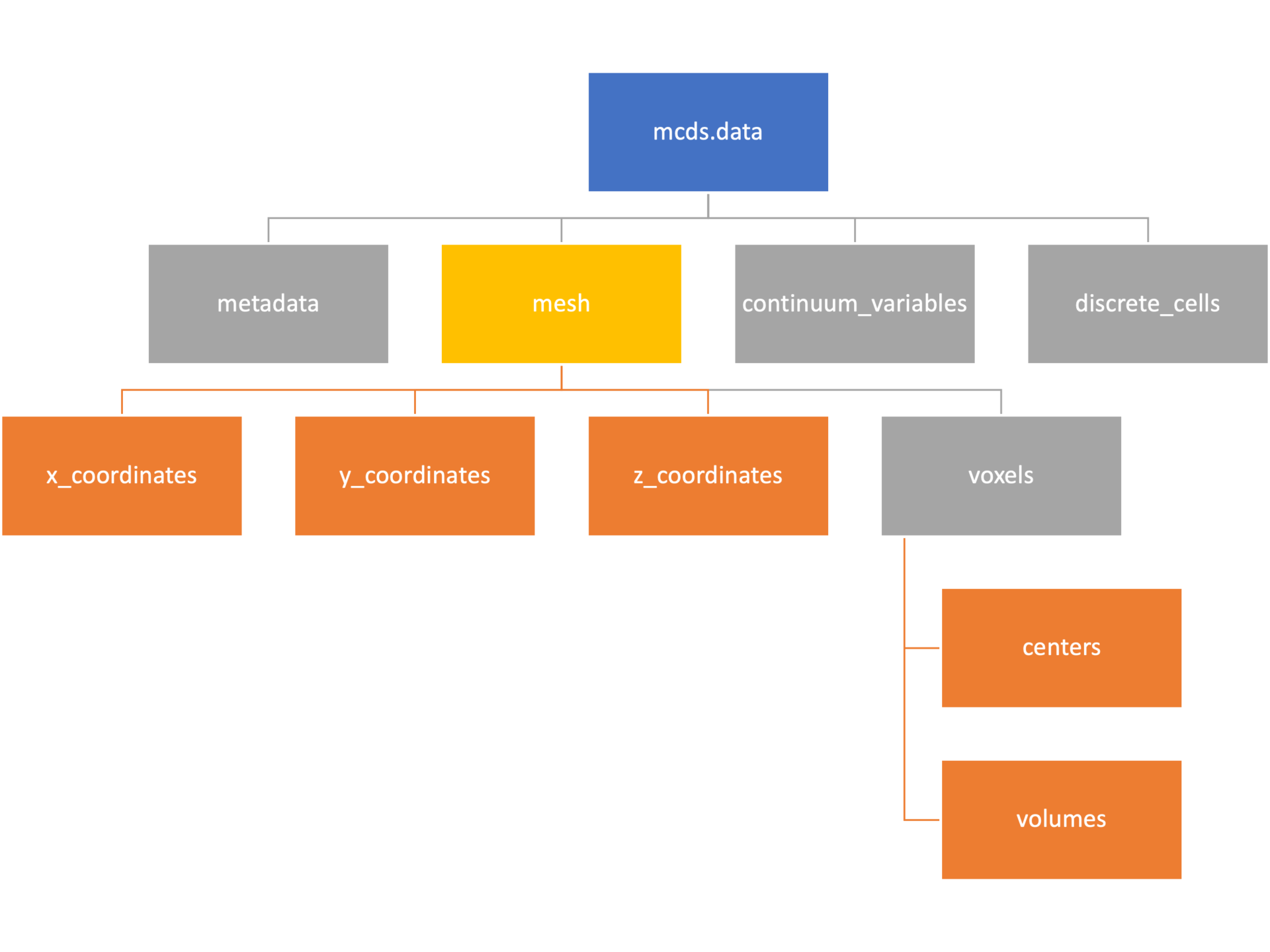
Continuum variables
The continuum_variables dictionary is the most complicated of the four. It contains subdictionaries that we access using the names of each of the chemicals in the microenvironment. In our toy example above, these are oxygen and my_chemical. If our model tracked diffusing oxygen, VEGF, and glucose, then the continuum_variables dictionary would contain a subdirectory for each of them.
For a particular chemical species in the microenvironment we have two more dictionaries called decay_rate and diffusion_coefficient, and a numpy array called data. The diffusion and decay dictionaries each complete the value stored as a scalar and the unit stored as a string. The numpy array contains the concentrations of the chemical in each voxel at this time and is the same shape as the meshgrids of the computational domain stored in the .data[‘mesh’] arrays.
# we need to know the names of the substrates to work with
# this data. We have a function to help us find them.
>>> mcds.get_substrate_names()
['oxygen', 'my_chemical']

# The diffusable chemical dictionaries are messy
# if we need to do a lot with them it might be easier
# to put them into their own instance
>>> oxy_dict = mcds.data['continuum_variables']['oxygen']
>>> oxy_dict['decay_rate']
{'value': 0.1, 'units': '1/min'}

# What we care about most is probably the numpy
# array of concentrations
>>> oxy_conc = oxy_dict['data']
>>> oxy_conc.shape
(75, 75, 75)

# Alternatively, we can get the same array with a function
>>> oxy_conc2 = mcds.get_concentrations('oxygen')
>>> oxy_conc2.shape
(75, 75, 75)

# We can also get the concentrations on a plane using the
# same function and supplying a z value to "slice through"
# note that right now the z_value must be an exact match
# for a plane of voxel centers, in the future we may add
# interpolation.
>>> oxy_plane = mcds.get_concentrations('oxygen', z_value=100.0)
>>> oxy_plane.shape
(75, 75)

# we can also find the concentration in a single voxel using the
# position of a point within that voxel. This will give us an
# array of all concentrations at that point.
>>> mcds.get_concentrations_at(x=0., y=550., z=0.)
array([17.94514446,  0.99113448])
Discrete Cells

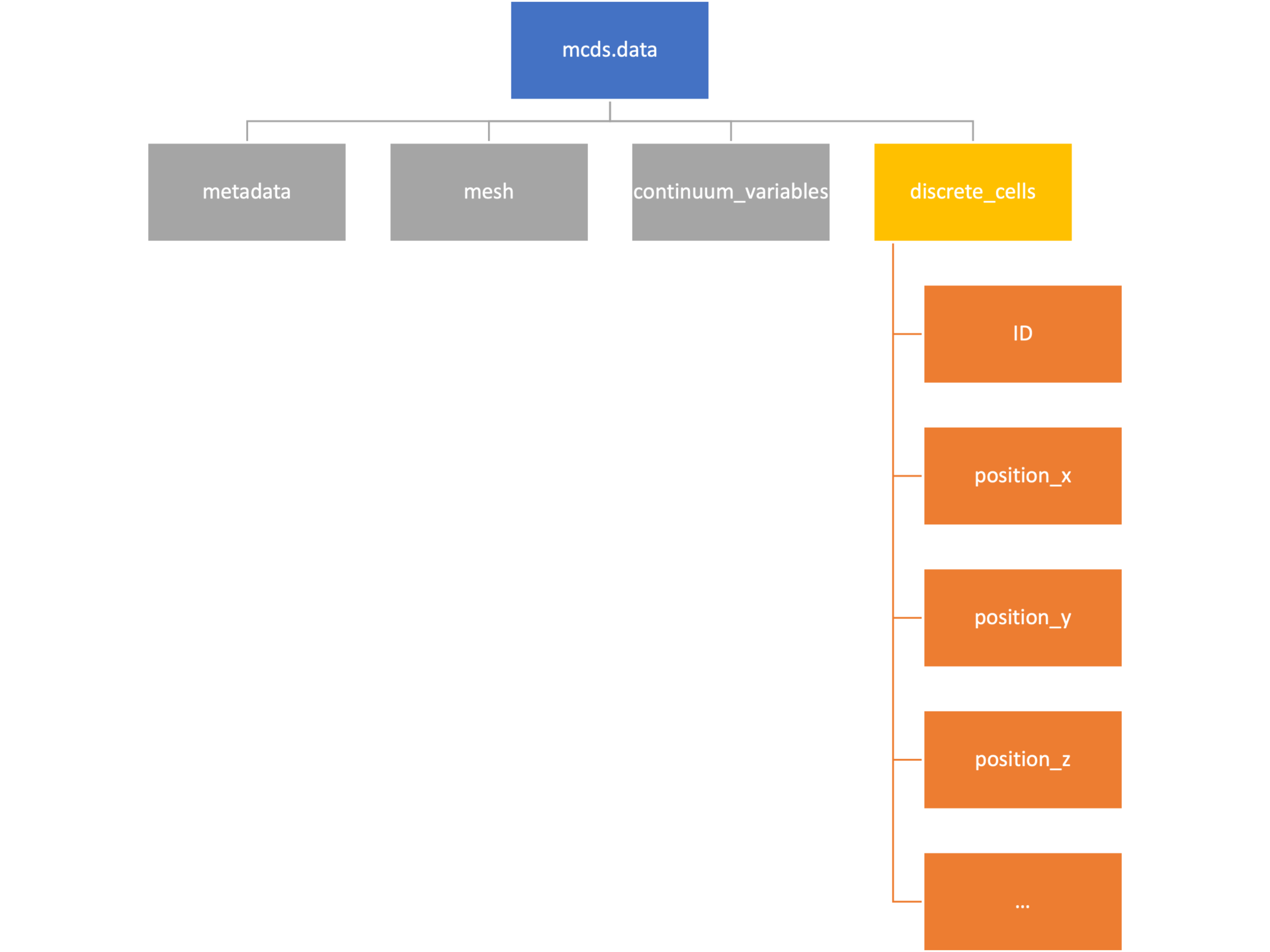
The discrete cells dictionary is relatively straightforward. It contains a number of numpy arrays that contain information regarding individual cells. These are all 1-dimensional arrays and each corresponds to one of the variables specified in the output*.xml file. With the default settings, these are:
- ID: unique integer that will identify the cell throughout its lifetime in the simulation
- position(_x, _y, _z): floating point positions for the cell in \(x\), \(y\), and \(z\) directions
- total_volume: total volume of the cell
- cell_type: integer label for the cell as used in PhysiCell
- cycle_model: integer label for the cell cycle model as used in PhysiCell
- current_phase: integer specification for which phase of the cycle model the cell is currently in
- elapsed_time_in_phase: time that cell has been in current phase of cell cycle model
- nuclear_volume: volume of cell nucleus
- cytoplasmic_volume: volume of cell cytoplasm
- fluid_fraction: proportion of the volume due to fliud
- calcified_fraction: proportion of volume consisting of calcified material
- orientation(_x, _y, _z): direction in which cell is pointing
- polarity:
- migration_speed: current speed of cell
- motility_vector(_x, _y, _z): current direction of movement of cell
- migration_bias: coefficient for stochastic movement (higher is “more deterministic”)
- motility_bias_direction(_x, _y, _z): direction of movement bias
- persistence_time: time in-between direction changes for cell
- motility_reserved:
# Extracting single variables is just like before
>>> cell_ids = mcds.data['discrete_cells']['ID']
>>> cell_ids.shape
(18595,)
>>> cell_ids[:4]
array([0., 1., 2., 3.])

# If we're clever we can extract 2D arrays
>>> cell_vec = np.zeros((cell_ids.shape[0], 3))
>>> vec_list = ['position_x', 'position_y', 'position_z']
>>> for i, lab in enumerate(vec_list):
...     cell_vec[:, i] = mcds.data['discrete_cells'][lab]
...
array([[ -69.72657128,  -39.02046405, -233.63178904],
       [ -69.84507464,  -22.71693265, -233.59277388],
       [ -69.84891462,   -6.04070516, -233.61816711],
       [ -69.845265  ,   10.80035554, -233.61667313]])

# We can get the list of all of the variables stored in this dictionary
>>> mcds.get_cell_variables()
['ID',
 'position_x',
 'position_y',
 'position_z',
 'total_volume',
 'cell_type',
 'cycle_model',
 'current_phase',
 'elapsed_time_in_phase',
 'nuclear_volume',
 'cytoplasmic_volume',
 'fluid_fraction',
 'calcified_fraction',
 'orientation_x',
 'orientation_y',
 'orientation_z',
 'polarity',
 'migration_speed',
 'motility_vector_x',
 'motility_vector_y',
 'motility_vector_z',
 'migration_bias',
 'motility_bias_direction_x',
 'motility_bias_direction_y',
 'motility_bias_direction_z',
 'persistence_time',
 'motility_reserved',
 'oncoprotein',
 'elastic_coefficient',
 'kill_rate',
 'attachment_lifetime',
 'attachment_rate']
# We can also get all of the cell data as a pandas DataFrame
>>> cell_df = mcds.get_cell_df()
>>> cell_df.head()
ID     position_x   position_y    position_z total_volume cell_type cycle_model ...
0.0   - 69.726571  - 39.020464  - 233.631789       2494.0       0.0         5.0 ...
1.0   - 69.845075  - 22.716933  - 233.592774       2494.0       0.0         5.0 ...
2.0   - 69.848915  - 6.040705   - 233.618167       2494.0       0.0         5.0 ...
3.0   - 69.845265    10.800356  - 233.616673       2494.0       0.0         5.0 ...
4.0   - 69.828161    27.324530  - 233.631579       2494.0       0.0         5.0 ...

# if we want to we can also get just the subset of cells that
# are in a specific voxel
>>> vox_df = mcds.get_cell_df_at(x=0.0, y=550.0, z=0.0)
>>> vox_df.iloc[:, :5]
             ID  position_x  position_y  position_z  total_volume
26718  228761.0    6.623617  536.709341   -1.282934   2454.814507
52736  270274.0   -7.990034  538.184921    9.648955   1523.386488
Examples
These examples will not be made using our toy dataset described above but will instead be made using a single timepoint dataset that can be found at:
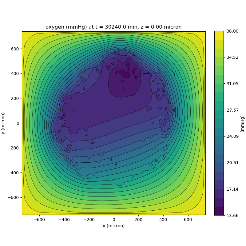
Substrate contour plot
One of the big advantages of working with PhysiCell data in python is that we have access to its plotting tools. For the sake of example let’s plot the partial pressure of oxygen throughout the computational domain along the \(z = 0\) plane. Once we’ve loaded our data by initializing a pyMCDS object, we can work entirely within python to produce the plot.
from pyMCDS import pyMCDS
import numpy as np
import matplotlib.pyplot as plt

# load data
mcds = pyMCDS('output00003696.xml', '../output')

# Set our z plane and get our substrate values along it
z_val = 0.00
plane_oxy = mcds.get_concentrations('oxygen', z_slice=z_val)

# Get the 2D mesh for contour plotting
xx, yy = mcds.get_mesh()

# We want to be able to control the number of contour levels so we
# need to do a little set up
num_levels = 21
min_conc = plane_oxy.min()
max_conc = plane_oxy.max()
my_levels = np.linspace(min_conc, max_conc, num_levels)

# set up the figure area and add data layers
fig, ax = plt.subplot()
cs = ax.contourf(xx, yy, plane_oxy, levels=my_levels)
ax.contour(xx, yy, plane_oxy, color='black', levels = my_levels,
           linewidths=0.5)

# Now we need to add our color bar
cbar1 = fig.colorbar(cs, shrink=0.75)
cbar1.set_label('mmHg')

# Let's put the time in to make these look nice
ax.set_aspect('equal')
ax.set_xlabel('x (micron)')
ax.set_ylabel('y (micron)')
ax.set_title('oxygen (mmHg) at t = {:.1f} {:s}, z = {:.2f} {:s}'.format(
                                        mcds.get_time(),
                                        mcds.data['metadata']['time_units'],
                                        z_val,
                                        mcds.data['metadata']['spatial_units'])

plt.show()
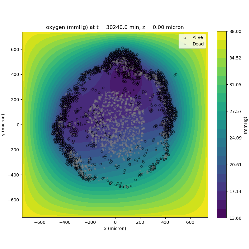
Adding a cells layer
We can also use pandas to do fairly complex selections of cells to add to our plots. Below we use pandas and the previous plot to add a cells layer.
from pyMCDS import pyMCDS
import numpy as np
import matplotlib.pyplot as plt

# load data
mcds = pyMCDS('output00003696.xml', '../output')

# Set our z plane and get our substrate values along it
z_val = 0.00
plane_oxy = mcds.get_concentrations('oxygen', z_slice=z_val)

# Get the 2D mesh for contour plotting
xx, yy = mcds.get_mesh()

# We want to be able to control the number of contour levels so we
# need to do a little set up
num_levels = 21
min_conc = plane_oxy.min()
max_conc = plane_oxy.max()
my_levels = np.linspace(min_conc, max_conc, num_levels)

# get our cells data and figure out which cells are in the plane
cell_df = mcds.get_cell_df()
ds = mcds.get_mesh_spacing()
inside_plane = (cell_df['position_z'] < z_val + ds) \ & (cell_df['position_z'] > z_val - ds)
plane_cells = cell_df[inside_plane]

# We're going to plot two types of cells and we want it to look nice
colors = ['black', 'grey']
sizes = [20, 8]
labels = ['Alive', 'Dead']

# set up the figure area and add microenvironment layer
fig, ax = plt.subplot()
cs = ax.contourf(xx, yy, plane_oxy, levels=my_levels)

# get our cells of interest
# alive_cells = plane_cells[plane_cells['cycle_model'] < 6]
# dead_cells = plane_cells[plane_cells['cycle_model'] > 6]
# -- for newer versions of PhysiCell
alive_cells = plane_cells[plane_cells['cycle_model'] < 100]
dead_cells = plane_cells[plane_cells['cycle_model'] >= 100]

# plot the cell layer
for i, plot_cells in enumerate((alive_cells, dead_cells)):
    ax.scatter(plot_cells['position_x'].values,
            plot_cells['position_y'].values,
            facecolor='none',
            edgecolors=colors[i],
            alpha=0.6,
            s=sizes[i],
            label=labels[i])

# Now we need to add our color bar
cbar1 = fig.colorbar(cs, shrink=0.75)
cbar1.set_label('mmHg')

# Let's put the time in to make these look nice
ax.set_aspect('equal')
ax.set_xlabel('x (micron)')
ax.set_ylabel('y (micron)')
ax.set_title('oxygen (mmHg) at t = {:.1f} {:s}, z = {:.2f} {:s}'.format(
                                        mcds.get_time(),
                                        mcds.data['metadata']['time_units'],
                                        z_val,
                                        mcds.data['metadata']['spatial_units'])
ax.legend(loc='upper right')

plt.show()
Future Direction
The first extension of this project will be timeseries functionality. This will provide similar data loading functionality but for a time series of MultiCell Digital Snapshots instead of simply one point in time.
PhysiCell Tools : PhysiCell-povwriter
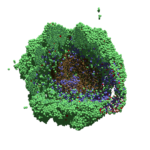
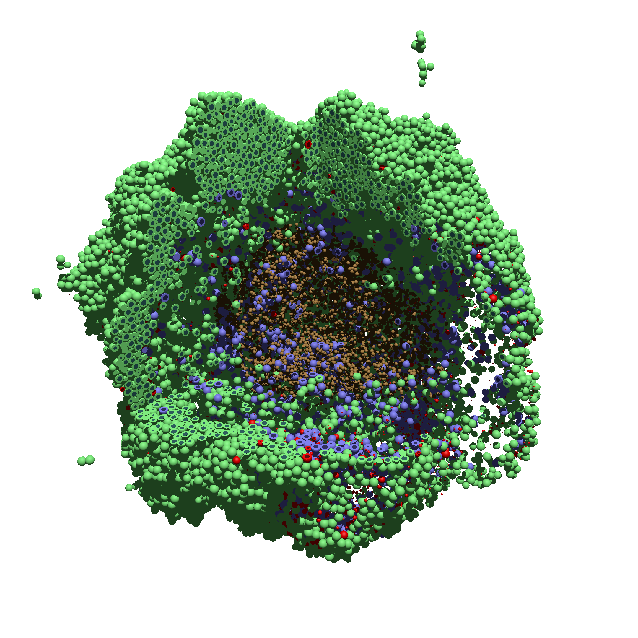
As PhysiCell matures, we are starting to turn our attention to better training materials and an ecosystem of open source PhysiCell tools. PhysiCell-povwriter is is designed to help transform your 3-D simulation results into 3-D visualizations like this one:
PhysiCell-povwriter transforms simulation snapshots into 3-D scenes that can be rendered into still images using POV-ray: an open source software package that uses raytracing to mimic the path of light from a source of illumination to a single viewpoint (a camera or an eye). The result is a beautifully rendered scene (at any resolution you choose) with very nice shading and lighting.
If you repeat this on many simulation snapshots, you can create an animation of your work.
What you’ll need
This workflow is entirely based on open source software:
- 3-D simulation data (likely stored in ./output from your project)
- PhysiCell-povwriter, available on GitHub at
- POV-ray, available at
- ImageMagick (optional, for image file conversions)
- mencoder (optional, for making compressed movies)
Setup
Building PhysiCell-povwriter
After you clone PhysiCell-povwriter or download its source from a release, you’ll need to compile it. In the project’s root directory, compile the project by:
make
(If you need to set up a C++ PhysiCell development environment, click here for OSX or here for Windows.)
Next, copy povwriter (povwriter.exe in Windows) to either the root directory of your PhysiCell project, or somewhere in your path. Copy ./config/povwriter-settings.xml to the ./config directory of your PhysiCell project.
Editing resolutions in POV-ray
PhysiCell-povwriter is intended for creating “square” images, but POV-ray does not have any pre-created square rendering resolutions out-of-the-box. However, this is straightforward to fix.
- Open POV-Ray
- Go to the “tools” menu and select “edit resolution INI file”
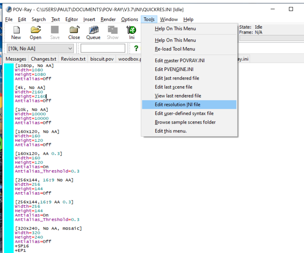
- At the top of the INI file (which opens for editing in POV-ray), make a new profile:
[1080x1080, AA]
Width=480
Height=480
Antialias=On
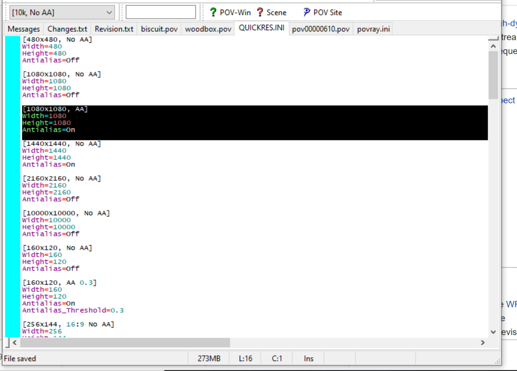
- Make similar profiles (with unique names) to suit your preferences. I suggest one at 480×480 (as a fast preview), another at 2160×2160, and another at 5000×5000 (because they will be absurdly high resolution). For example:
[2160x2160 no AA]
Width=2160
Height=2160
Antialias=Off
You can optionally make more profiles with antialiasing on (which provides some smoothing for areas of high detail), but you’re probably better off just rendering without antialiasing at higher resolutions and the scaling the image down as needed. Also, rendering without antialiasing will be faster.
- Once done making profiles, save and exit POV-Ray.
- The next time you open POV-Ray, your new resolution profiles will be available in the lefthand dropdown box.


Configuring PhysiCell-povwriter
Once you have copied povwriter-settings.xml to your project’s config file, open it in a text editor. Below, we’ll show the different settings.
Camera settings
<camera>
	<distance_from_origin units="micron">1500</distance_from_origin>
	<xy_angle>3.92699081699</xy_angle> <!-- 5*pi/4 -->
	<yz_angle>1.0471975512</yz_angle> <!-- pi/3 -->
</camera>
For simplicity, PhysiCell-POVray (currently) always aims the camera towards the origin (0,0,0), with “up” towards the positive z-axis. distance_from_origin sets how far the camera is placed from the origin. xy_angle sets the angle \(\theta\) from the positive x-axis in the xy-plane. yz_angle sets the angle \(\phi\) from the positive z-axis in the yz-plane. Both angles are in radians.
Options
<options>
	<use_standard_colors>true</use_standard_colors>
	<nuclear_offset units="micron">0.1</nuclear_offset>
	<cell_bound units="micron">750</cell_bound>
	<threads>8</threads>
</options>
use_standard_colors (if set to true) uses a built-in “paint-by-numbers” color scheme, where each cell type (identified with an integer) gets XML-defined colors for live, apoptotic, and dead cells. More on this below. If use_standard_colors is set to false, then PhysiCell-povwriter uses the my_pigment_and_finish_function in ./custom_modules/povwriter.cpp to color cells.
The nuclear_offset is a small additional height given to nuclei when cropping to avoid visual artifacts when rendering (which can cause some “tearing” or “bleeding” between the rendered nucleus and cytoplasm). cell_bound is used for leaving some cells out of bound: any cell with |x|, |y|, or |z| exceeding cell_bound will not be rendered. threads is used for parallelizing on multicore processors; note that it only speeds up povwriter if you are converting multiple PhysiCell outputs to povray files.
Save
<save> <!-- done -->
	<folder>output</folder> <!-- use . for root -->
	<filebase>output</filebase>
	<time_index>3696</time_index>
</save>
Use folder to tell PhysiCell-povwriter where the data files are stored. Use filebase to tell how the outputs are named. Typically, they have the form output########_cells_physicell.mat; in this case, the filebase is output. Lastly, use time_index to set the output number. For example if your file is output00000182_cells_physicell.mat, then filebase = output and time_index = 182.
Below, we’ll see how to specify ranges of indices at the command line, which would supersede the time_index given here in the XML.
Clipping planes
PhysiCell-povwriter uses clipping planes to help create cutaway views of the simulations. By default, 3 clipping planes are used to cut out an octant of the viewing area.
Recall that a plane can be defined by its normal vector n and a point p on the plane. With these, the plane can be defined as all points x satisfying
\[ \left( \vec{x} -\vec{p} \right) \cdot \vec{n} = 0 \]
These are then written out as a plane equation
\[ a x + by + cz + d = 0, \]
where
\[ (a,b,c) = \vec{n} \hspace{.5in} \textrm{ and } \hspace{0.5in} d = \: – \vec{n} \cdot \vec{p}. \]
As of Version 1.0.0, we are having some difficulties with clipping planes that do not pass through the origin (0,0,0), for which \( d = 0 \).
In the config file, these planes are written as \( (a,b,c,d) \):
<clipping_planes> <!-- done -->
	<clipping_plane>0,-1,0,0</clipping_plane>
	<clipping_plane>-1,0,0,0</clipping_plane>
	<clipping_plane>0,0,1,0</clipping_plane>
</clipping_planes>
Note that cells “behind” the plane (where \( ( \vec{x} – \vec{p} ) \cdot \vec{n} \le 0 \)) are rendered, and cells in “front” of the plane (where \( (\vec{x}-\vec{p}) \cdot \vec{n} > 0 \)) are not rendered. Cells that intersect the plane are partially rendered (using constructive geometry via union and intersection commands in POV-ray).
Cell color definitions
Within <cell_color_definitions>, you’ll find multiple <cell_colors> blocks, each of which defines the live, dead, and necrotic colors for a specific cell type (with the type ID indicated in the attribute). These colors are only applied if use_standard_colors is set to true in options. See above.
The live colors are given as two rgb (red,green,blue) colors for the cytoplasm and nucleus of live cells. Each element of this triple can range from 0 to 1, and not from 0 to 255 as in many raw image formats. Next, finish specifies ambient (how much highly-scattered background ambient light illuminates the cell), diffuse (how well light rays can illuminate the surface), and specular (how much of a shiny reflective splotch the cell gets).
See the POV-ray documentation for for information on the finish.
This is repeated to give the apoptotic and necrotic colors for the cell type.
<cell_colors type="0">
	<live>
		<cytoplasm>.25,1,.25</cytoplasm> <!-- red,green,blue -->
		<nuclear>0.03,0.125</nuclear>
		<finish>0.05,1,0.1</finish> <!-- ambient,diffuse,specular -->
	</live>
	<apoptotic>
		<cytoplasm>1,0,0</cytoplasm> <!-- red,green,blue -->
		<nuclear>0.125,0,0</nuclear>
		<finish>0.05,1,0.1</finish> <!-- ambient,diffuse,specular -->
	</apoptotic>
	<necrotic>
		<cytoplasm>1,0.5412,0.1490</cytoplasm> <!-- red,green,blue -->
		<nuclear>0.125,0.06765,0.018625</nuclear>
		<finish>0.01,0.5,0.1</finish> <!-- ambient,diffuse,specular -->
	</necrotic>
</cell_colors>
Use multiple cell_colors blocks (each with type corresponding to the integer cell type) to define the colors of multiple cell types.
Using PhysiCell-povwriter
Use by the XML configuration file alone
The simplest syntax:
physicell$ ./povwriter
(Windows users: povwriter or povwriter.exe) will process ./config/povwriter-settings.xml and convert the single indicated PhysiCell snapshot to a .pov file.
If you run POV-writer with the default configuration file in the povwriter structure (with the supplied sample data), it will render time index 3696 from the immunotherapy example in our 2018 PhysiCell Method Paper:
physicell$ ./povwriter

povwriter version 1.0.0
================================================================================

Copyright (c) Paul Macklin 2019, on behalf of the PhysiCell project
OSI License: BSD-3-Clause (see LICENSE.txt)

Usage:
================================================================================
povwriter : run povwriter with config file ./config/settings.xml

povwriter FILENAME.xml : run povwriter with config file FILENAME.xml

povwriter x:y:z : run povwriter on data in FOLDER with indices from x
to y in incremenets of z

Example: ./povwriter 0:2:10 processes files:
./FOLDER/FILEBASE00000000_physicell_cells.mat
./FOLDER/FILEBASE00000002_physicell_cells.mat
...
./FOLDER/FILEBASE00000010_physicell_cells.mat
(See the config file to set FOLDER and FILEBASE)

povwriter x1,...,xn : run povwriter on data in FOLDER with indices x1,...,xn

Example: ./povwriter 1,3,17 processes files:
./FOLDER/FILEBASE00000001_physicell_cells.mat
./FOLDER/FILEBASE00000003_physicell_cells.mat
./FOLDER/FILEBASE00000017_physicell_cells.mat
(Note that there are no spaces.)
(See the config file to set FOLDER and FILEBASE)

Code updates at https://github.com/PhysiCell-Tools/PhysiCell-povwriter

Tutorial & documentation at http://MathCancer.org/blog/povwriter
================================================================================

Using config file ./config/povwriter-settings.xml ...
Using standard coloring function ...
Found 3 clipping planes ...
Found 2 cell color definitions ...
Processing file ./output/output00003696_cells_physicell.mat...
Matrix size: 32 x 66978
Creating file pov00003696.pov for output ...
Writing 66978 cells ...
done!

Done processing all 1 files!
The result is a single POV-ray file (pov00003696.pov) in the root directory.
Now, open that file in POV-ray (double-click the file if you are in Windows), choose one of your resolutions in your lefthand dropdown (I’ll choose 2160×2160 no antialiasing), and click the green “run” button.
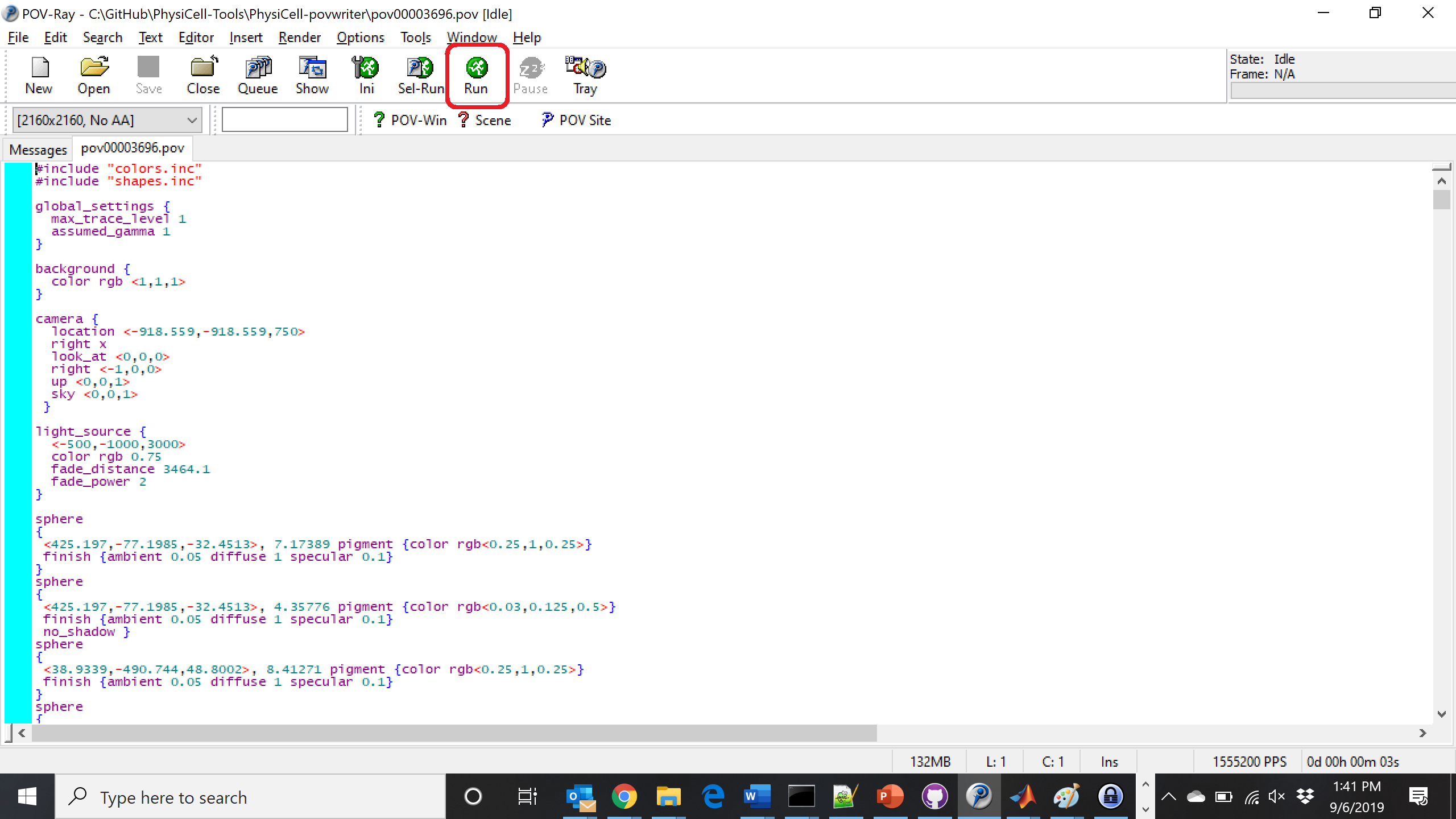
You can watch the image as it renders. The result should be a PNG file (named pov00003696.png) that looks like this:
Using command-line options to process multiple times (option #1)
Now, suppose we have more outputs to process. We still state most of the options in the XML file as above, but now we also supply a command-line argument in the form of start:interval:end. If you’re still in the povwriter project, note that we have some more sample data there. Let’s grab and process it:
physicell$ cd output
physicell$ unzip more_samples.zip
Archive: more_samples.zip
inflating: output00000000_cells_physicell.mat
inflating: output00000001_cells_physicell.mat
inflating: output00000250_cells_physicell.mat
inflating: output00000300_cells_physicell.mat
inflating: output00000500_cells_physicell.mat
inflating: output00000750_cells_physicell.mat
inflating: output00001000_cells_physicell.mat
inflating: output00001250_cells_physicell.mat
inflating: output00001500_cells_physicell.mat
inflating: output00001750_cells_physicell.mat
inflating: output00002000_cells_physicell.mat
inflating: output00002250_cells_physicell.mat
inflating: output00002500_cells_physicell.mat
inflating: output00002750_cells_physicell.mat
inflating: output00003000_cells_physicell.mat
inflating: output00003250_cells_physicell.mat
inflating: output00003500_cells_physicell.mat
inflating: output00003696_cells_physicell.mat

physicell$ ls

citation and license.txt
more_samples.zip
output00000000_cells_physicell.mat
output00000001_cells_physicell.mat
output00000250_cells_physicell.mat
output00000300_cells_physicell.mat
output00000500_cells_physicell.mat
output00000750_cells_physicell.mat
output00001000_cells_physicell.mat
output00001250_cells_physicell.mat
output00001500_cells_physicell.mat
output00001750_cells_physicell.mat
output00002000_cells_physicell.mat
output00002250_cells_physicell.mat
output00002500_cells_physicell.mat
output00002750_cells_physicell.mat
output00003000_cells_physicell.mat
output00003250_cells_physicell.mat
output00003500_cells_physicell.mat
output00003696.xml
output00003696_cells_physicell.mat
Let’s go back to the parent directory and run povwriter:
physicell$ ./povwriter 0:250:3500

povwriter version 1.0.0
================================================================================

Copyright (c) Paul Macklin 2019, on behalf of the PhysiCell project
OSI License: BSD-3-Clause (see LICENSE.txt)

Usage:
================================================================================
povwriter : run povwriter with config file ./config/settings.xml

povwriter FILENAME.xml : run povwriter with config file FILENAME.xml

povwriter x:y:z : run povwriter on data in FOLDER with indices from x
to y in incremenets of z

Example: ./povwriter 0:2:10 processes files:
./FOLDER/FILEBASE00000000_physicell_cells.mat
./FOLDER/FILEBASE00000002_physicell_cells.mat
...
./FOLDER/FILEBASE00000010_physicell_cells.mat
(See the config file to set FOLDER and FILEBASE)

povwriter x1,...,xn : run povwriter on data in FOLDER with indices x1,...,xn

Example: ./povwriter 1,3,17 processes files:
./FOLDER/FILEBASE00000001_physicell_cells.mat
./FOLDER/FILEBASE00000003_physicell_cells.mat
./FOLDER/FILEBASE00000017_physicell_cells.mat
(Note that there are no spaces.)
(See the config file to set FOLDER and FILEBASE)

Code updates at https://github.com/PhysiCell-Tools/PhysiCell-povwriter

Tutorial & documentation at http://MathCancer.org/blog/povwriter
================================================================================

Using config file ./config/povwriter-settings.xml ...
Using standard coloring function ...
Found 3 clipping planes ...
Found 2 cell color definitions ...
Matrix size: 32 x 18317
Processing file ./output/output00000000_cells_physicell.mat...
Creating file pov00000000.pov for output ...
Writing 18317 cells ...
Processing file ./output/output00002000_cells_physicell.mat...
Matrix size: 32 x 33551
Creating file pov00002000.pov for output ...
Writing 33551 cells ...
Processing file ./output/output00002500_cells_physicell.mat...
Matrix size: 32 x 43440
Creating file pov00002500.pov for output ...
Writing 43440 cells ...
Processing file ./output/output00001500_cells_physicell.mat...
Matrix size: 32 x 40267
Creating file pov00001500.pov for output ...
Writing 40267 cells ...
Processing file ./output/output00003000_cells_physicell.mat...
Matrix size: 32 x 56659
Creating file pov00003000.pov for output ...
Writing 56659 cells ...
Processing file ./output/output00001000_cells_physicell.mat...
Matrix size: 32 x 74057
Creating file pov00001000.pov for output ...
Writing 74057 cells ...
Processing file ./output/output00003500_cells_physicell.mat...
Matrix size: 32 x 66791
Creating file pov00003500.pov for output ...
Writing 66791 cells ...
Processing file ./output/output00000500_cells_physicell.mat...
Matrix size: 32 x 114316
Creating file pov00000500.pov for output ...
Writing 114316 cells ...
done!

Processing file ./output/output00000250_cells_physicell.mat...
Matrix size: 32 x 75352
Creating file pov00000250.pov for output ...
Writing 75352 cells ...
done!

Processing file ./output/output00002250_cells_physicell.mat...
Matrix size: 32 x 37959
Creating file pov00002250.pov for output ...
Writing 37959 cells ...
done!

Processing file ./output/output00001750_cells_physicell.mat...
Matrix size: 32 x 32358
Creating file pov00001750.pov for output ...
Writing 32358 cells ...
done!

Processing file ./output/output00002750_cells_physicell.mat...
Matrix size: 32 x 49658
Creating file pov00002750.pov for output ...
Writing 49658 cells ...
done!

Processing file ./output/output00003250_cells_physicell.mat...
Matrix size: 32 x 63546
Creating file pov00003250.pov for output ...
Writing 63546 cells ...
done!

done!

done!

done!

Processing file ./output/output00001250_cells_physicell.mat...
Matrix size: 32 x 54771
Creating file pov00001250.pov for output ...
Writing 54771 cells ...
done!

done!

done!

done!

Processing file ./output/output00000750_cells_physicell.mat...
Matrix size: 32 x 97642
Creating file pov00000750.pov for output ...
Writing 97642 cells ...
done!

done!

Done processing all 15 files!
Notice that the output appears a bit out of order. This is normal: povwriter is using 8 threads to process 8 files at the same time, and sending some output to the single screen. Since this is all happening simultaneously, it’s a bit jumbled (and non-sequential). Don’t panic. You should now have created pov00000000.pov, pov00000250.pov, … , pov00003500.pov.
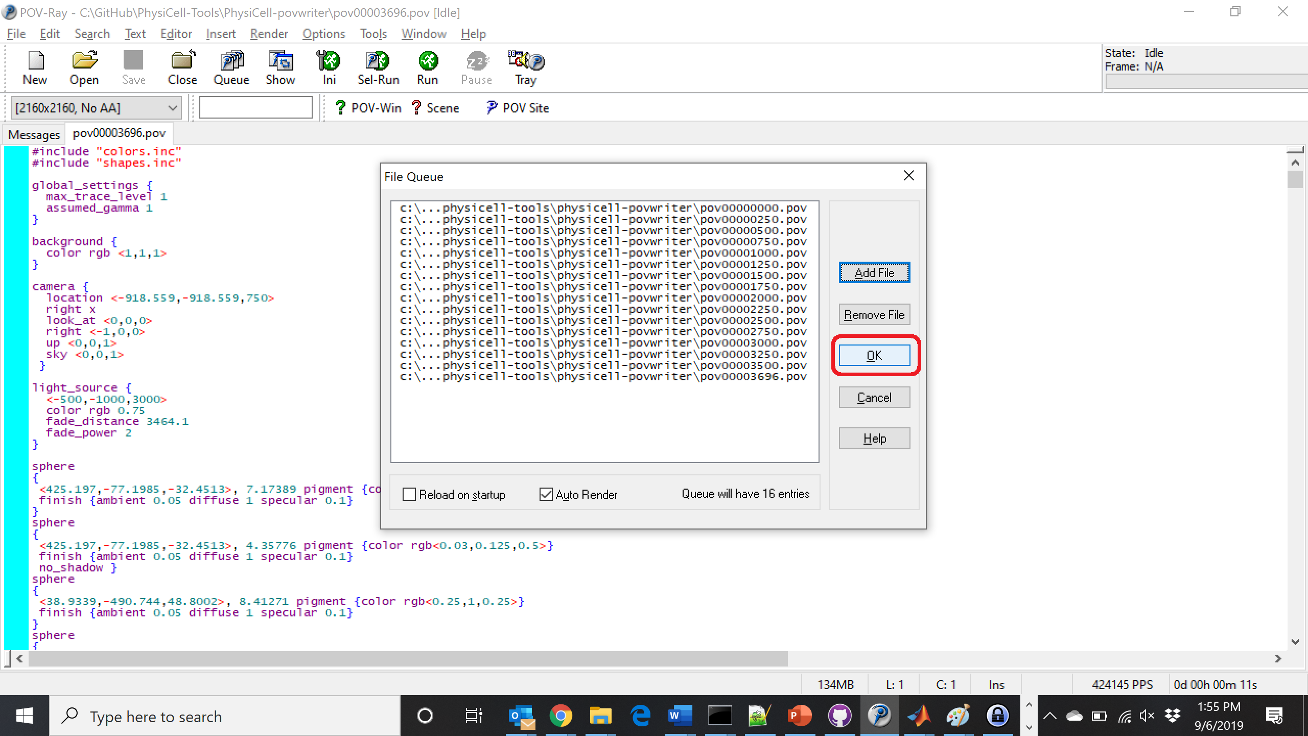
Now, go into POV-ray, and choose “queue.” Click “Add File” and select all 15 .pov files you just created:
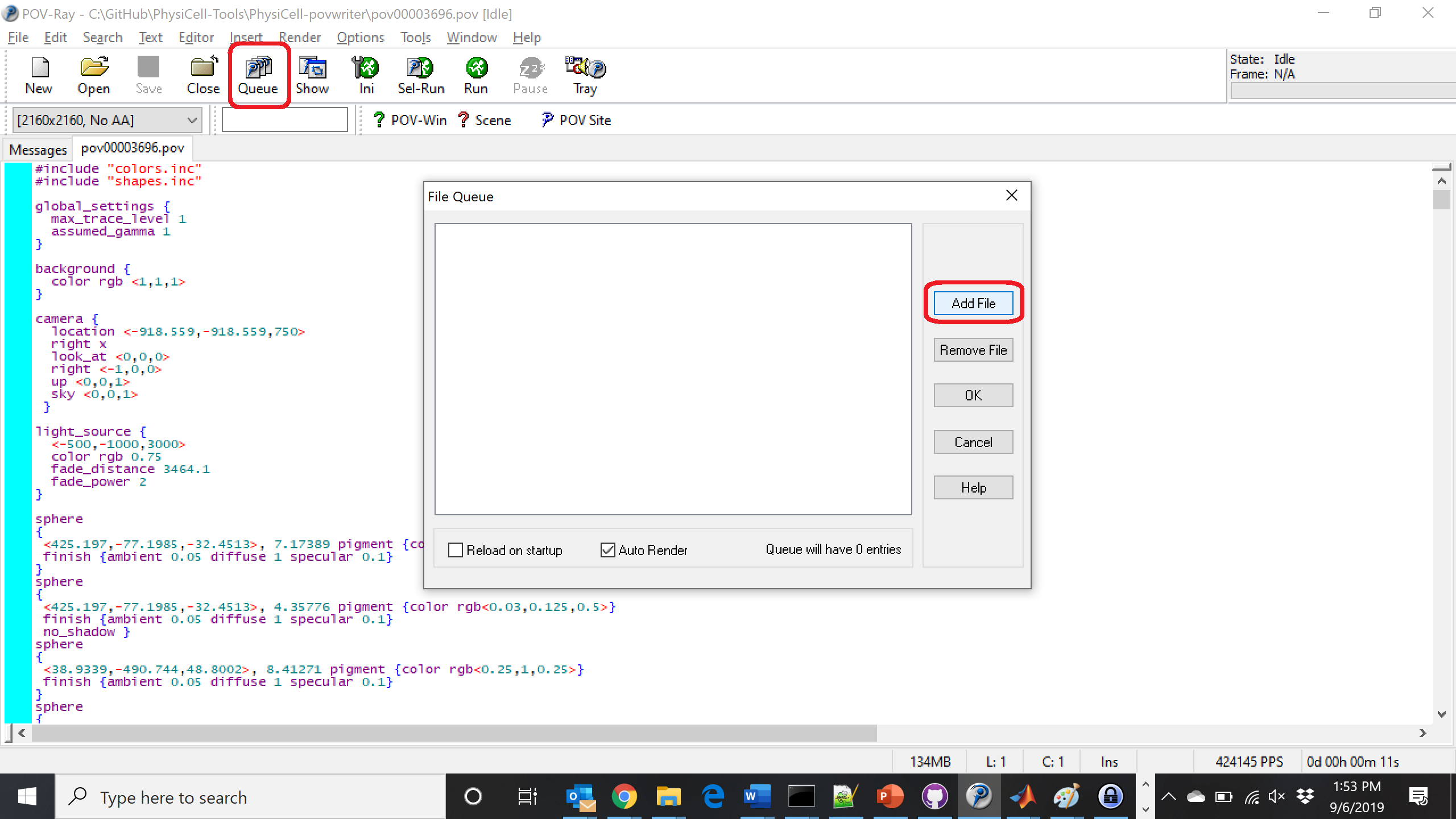
Hit “OK” to let it render all the povray files to create PNG files (pov00000000.png, … , pov00003500.png).
Using command-line options to process multiple times (option #2)
You can also give a list of indices. Here’s how we render time indices 250, 1000, and 2250:
physicell$ ./povwriter 250,1000,2250

povwriter version 1.0.0
================================================================================

Copyright (c) Paul Macklin 2019, on behalf of the PhysiCell project
OSI License: BSD-3-Clause (see LICENSE.txt)

Usage:
================================================================================
povwriter : run povwriter with config file ./config/settings.xml

povwriter FILENAME.xml : run povwriter with config file FILENAME.xml

povwriter x:y:z : run povwriter on data in FOLDER with indices from x
to y in incremenets of z

Example: ./povwriter 0:2:10 processes files:
./FOLDER/FILEBASE00000000_physicell_cells.mat
./FOLDER/FILEBASE00000002_physicell_cells.mat
...
./FOLDER/FILEBASE00000010_physicell_cells.mat
(See the config file to set FOLDER and FILEBASE)

povwriter x1,...,xn : run povwriter on data in FOLDER with indices x1,...,xn

Example: ./povwriter 1,3,17 processes files:
./FOLDER/FILEBASE00000001_physicell_cells.mat
./FOLDER/FILEBASE00000003_physicell_cells.mat
./FOLDER/FILEBASE00000017_physicell_cells.mat
(Note that there are no spaces.)
(See the config file to set FOLDER and FILEBASE)

Code updates at https://github.com/PhysiCell-Tools/PhysiCell-povwriter

Tutorial & documentation at http://MathCancer.org/blog/povwriter
================================================================================

Using config file ./config/povwriter-settings.xml ...
Using standard coloring function ...
Found 3 clipping planes ...
Found 2 cell color definitions ...
Processing file ./output/output00002250_cells_physicell.mat...
Matrix size: 32 x 37959
Creating file pov00002250.pov for output ...
Writing 37959 cells ...
Processing file ./output/output00001000_cells_physicell.mat...
Matrix size: 32 x 74057
Creating file pov00001000.pov for output ...
Processing file ./output/output00000250_cells_physicell.mat...
Matrix size: 32 x 75352
Writing 74057 cells ...
Creating file pov00000250.pov for output ...
Writing 75352 cells ...
done!

done!

done!

Done processing all 3 files!
This will create files pov00000250.pov, pov00001000.pov, and pov00002250.pov. Render them in POV-ray just as before.
Advanced options (at the source code level)
If you set use_standard_colors to false, povwriter uses the function my_pigment_and_finish_function (at the end of ./custom_modules/povwriter.cpp). Make sure that you set colors.cyto_pigment (RGB) and colors.nuclear_pigment (also RGB). The source file in povwriter has some hinting on how to write this. Note that the XML files saved by PhysiCell have a legend section that helps you do determine what is stored in each column of the matlab file.
Optional postprocessing
Image conversion / manipulation with ImageMagick
Suppose you want to convert the PNG files to JPEGs, and scale them down to 60% of original size. That’s very straightforward in ImageMagick:
physicell$ magick mogrify -format jpg -resize 60% pov*.png
Creating an animated GIF with ImageMagick
Suppose you want to create an animated GIF based on your images. I suggest first converting to JPG (see above) and then using ImageMagick again. Here, I’m adding a 20 ms delay between frames:
physicell$ magick convert -delay 20 *.jpg out.gif
Here’s the result:
Creating a compressed movie with Mencoder
Syntax coming later.
Closing thoughts and future work
In the future, we will probably allow more control over the clipping planes and a bit more debugging on how to handle planes that don’t pass through the origin. (First thoughts: we need to change how we use union and intersection commands in the POV-ray outputs.)
We should also look at adding some transparency for the cells. I’d prefer something like rgba (red-green-blue-alpha), but POV-ray uses filters and transmission, and we want to make sure to get it right.
Lastly, it would be nice to find a balance between the current very simple camera setup and better control.
Thanks for reading this PhysiCell Friday tutorial! Please do give PhysiCell at try (at http://PhysiCell.org) and read the method paper at PLoS Computational Biology.
Setting up the PhysiCell microenvironment with XML
As of release 1.6.0, users can define all the chemical substrates in the microenvironment with an XML configuration file. (These are stored by default in ./config/. The default parameter file is ./config/PhysiCell_settings.xml.) This should make it much easier to set up the microenvironment (previously required a lot of manual C++), as well as make it easier to change parameters and initial conditions.
In release 1.7.0, users gained finer grained control on Dirichlet conditions: individual Dirichlet conditions can be enabled or disabled for each individual diffusing substrate on each individual boundary. See details below.
This tutorial will show you the key techniques to use these features. (See the User_Guide for full documentation.) First, let’s create a barebones 2D project by populating the 2D template project. In a terminal shell in your root PhysiCell directory, do this:
make template2D
We will use this 2D project template for the remainder of the tutorial. We assume you already have a working copy of PhysiCell installed, version 1.6.0 or later. (If not, visit the PhysiCell tutorials to find installation instructions for your operating system.) You will need version 1.7.0 or later to control Dirichlet conditions on individual boundaries.
You can download the latest version of PhysiCell at:
- GitHub: https://github.com/MathCancer/PhysiCell/releases
- SourceForge: https://sourceforge.net/projects/physicell/files/latest/download
Microenvironment setup in the XML configuration file
Next, let’s look at the parameter file. In your text editor of choice, open up ./config/PhysiCell_settings.xml, and browse down to <microenvironment_setup>:
<microenvironment_setup>
	<variable name="oxygen" units="mmHg" ID="0">
		<physical_parameter_set>
			<diffusion_coefficient units="micron^2/min">100000.0</diffusion_coefficient>
			<decay_rate units="1/min">0.1</decay_rate>
		</physical_parameter_set>
		<initial_condition units="mmHg">38.0</initial_condition>
		<Dirichlet_boundary_condition units="mmHg" enabled="true">38.0</Dirichlet_boundary_condition>
	</variable>

	<options>
		<calculate_gradients>false</calculate_gradients>
		<track_internalized_substrates_in_each_agent>false</track_internalized_substrates_in_each_agent>
		<!-- not yet supported -->
		<initial_condition type="matlab" enabled="false">
			<filename>./config/initial.mat</filename>
		</initial_condition>
		<!-- not yet supported -->
		<dirichlet_nodes type="matlab" enabled="false">
			<filename>./config/dirichlet.mat</filename>
		</dirichlet_nodes>
	</options>
</microenvironment_setup>
Notice a few trends:
- The <variable> XML element (tag) is used to define a chemical substrate in the microenvironment. The attributes say that it is named oxygen, and the units of measurement are mmHg. Notice also that the ID is 0: this unique integer identifier helps for finding and accessing the substrate within your PhysiCell project. Make sure your first substrate ID is 0, since C++ starts indexing at 0.
- Within the <variable> block, we set the properties of this substrate:
- <diffusion_coefficient> sets the (uniform) diffusion constant for the substrate.
- <decay_rate> is the substrate’s background decay rate.
- <initial_condition> is the value the substrate will be (uniformly) initialized to throughout the domain.
- <Dirichlet_boundary_condition> is the value the substrate will be set to along the outer computational boundary throughout the simulation, if you set enabled=true. If enabled=false, then PhysiCell (via BioFVM) will use Neumann (zero flux) conditions for that substrate.
- The <options> element helps configure other simulation behaviors:
- Use <calculate_gradients> to control whether PhysiCell computes all chemical gradients at each time step. Set this to true to enable accurate gradients (e.g., for chemotaxis).
- Use <track_internalized_substrates_in_each_agent> to enable or disable the PhysiCell feature of actively tracking the total amount of internalized substrates in each individual agent. Set this to true to enable the feature.
- <initial_condition> is reserved for a future release where we can specify non-uniform initial conditions as an external file (e.g., a CSV or Matlab file). This is not yet supported.
- <dirichlet_nodes> is reserved for a future release where we can specify Dirchlet nodes at any location in the simulation domain with an external file. This will be useful for irregular domains, but it is not yet implemented.
Note that PhysiCell does not convert units. The units attributes are helpful for clarity between users and developers, to ensure that you have worked in consistent length and time units. By default, PhysiCell uses minutes for all time units, and microns for all spatial units.
Changing an existing substrate
Let’s modify the oxygen variable to do the following:
- Change the diffusion coefficient to 120000 \(\mu\mathrm{m}^2 / \mathrm{min}\)
- Change the initial condition to 40 mmHg
- Change the oxygen Dirichlet boundary condition to 42.7 mmHg
- Enable gradient calculations
If you modify the appropriate fields in the <microenvironment_setup> block, it should look like this:
<microenvironment_setup>
	<variable name="oxygen" units="mmHg" ID="0">
		<physical_parameter_set>
			<diffusion_coefficient units="micron^2/min">120000.0</diffusion_coefficient>
			<decay_rate units="1/min">0.1</decay_rate>
		</physical_parameter_set>
		<initial_condition units="mmHg">40.0</initial_condition>
		<Dirichlet_boundary_condition units="mmHg" enabled="true">42.7</Dirichlet_boundary_condition>
	</variable>

	<options>
		<calculate_gradients>true</calculate_gradients>
		<track_internalized_substrates_in_each_agent>false</track_internalized_substrates_in_each_agent>
		<!-- not yet supported -->
		<initial_condition type="matlab" enabled="false">
			<filename>./config/initial.mat</filename>
		</initial_condition>
		<!-- not yet supported -->
		<dirichlet_nodes type="matlab" enabled="false">
			<filename>./config/dirichlet.mat</filename>
		</dirichlet_nodes>
	</options>
</microenvironment_setup>
Adding a new diffusing substrate
Let’s add a new dimensionless substrate glucose with the following:
- Diffusion coefficient is 18000 \(\mu\mathrm{m}^2 / \mathrm{min}\)
- No decay rate
- The initial condition is 1 (dimensionless)
- Neumann (no flux) boundary conditions
To add the new variable, I suggest copying an existing variable (in this case, oxygen) and modifying to:
- change the name and units throughout
- increase the ID by one
- write in the appropriate initial and boundary conditions
If you modify the appropriate fields in the <microenvironment_setup> block, it should look like this:
<microenvironment_setup>
	<variable name="oxygen" units="mmHg" ID="0">
		<physical_parameter_set>
			<diffusion_coefficient units="micron^2/min">120000.0</diffusion_coefficient>
			<decay_rate units="1/min">0.1</decay_rate>
		</physical_parameter_set>
		<initial_condition units="mmHg">40.0</initial_condition>
		<Dirichlet_boundary_condition units="mmHg" enabled="true">42.7</Dirichlet_boundary_condition>
	</variable>

	<variable name="glucose" units="dimensionless" ID="1">
		<physical_parameter_set>
			<diffusion_coefficient units="micron^2/min">18000.0</diffusion_coefficient>
			<decay_rate units="1/min">0.0</decay_rate>
		</physical_parameter_set>
		<initial_condition units="dimensionless">1</initial_condition>
		<Dirichlet_boundary_condition units="dimensionless" enabled="false">0</Dirichlet_boundary_condition>
	</variable>

	<options>
		<calculate_gradients>true</calculate_gradients>
		<track_internalized_substrates_in_each_agent>false</track_internalized_substrates_in_each_agent>
		<!-- not yet supported -->
		<initial_condition type="matlab" enabled="false">
			<filename>./config/initial.mat</filename>
		</initial_condition>
		<!-- not yet supported -->
		<dirichlet_nodes type="matlab" enabled="false">
			<filename>./config/dirichlet.mat</filename>
		</dirichlet_nodes>
	</options>
</microenvironment_setup>
Controlling Dirichlet conditions on individual boundaries
In Version 1.7.0, we introduced the ability to control the Dirichlet conditions for each individual boundary for each substrate. The examples above apply (enable) or disable the same condition on each boundary with the same boundary value.
Suppose that we want to set glucose so that the Dirichlet condition is enabled on the bottom z boundary (with value 1) and the left and right x boundaries (with value 0.5) and disabled on all other boundaries. We modify the variable block by adding the optional Dirichlet_options block:
<variable name="glucose" units="dimensionless" ID="1">
	<physical_parameter_set>
		<diffusion_coefficient units="micron^2/min">18000.0</diffusion_coefficient>
		<decay_rate units="1/min">0.0</decay_rate>
	</physical_parameter_set>
	<initial_condition units="dimensionless">1</initial_condition>
	<Dirichlet_boundary_condition units="dimensionless" enabled="true">0</Dirichlet_boundary_condition>
	<Dirichlet_options>
		<boundary_value ID="xmin" enabled="true">0.5</boundary_value>
		<boundary_value ID="xmax" enabled="true">0.5</boundary_value>
		<boundary_value ID="ymin" enabled="false">0.5</boundary_value>
		<boundary_value ID="ymin" enabled="false">0.5</boundary_value>
		<boundary_value ID="zmin" enabled="true">1.0</boundary_value>
		<boundary_value ID="zmax" enabled="false">0.5</boundary_value>
	</Dirichlet_options>
</variable>
Notice a few things:
- The Dirichlet_boundary_condition element has its enabled attribute set to true
- The Dirichlet condition is set under any individual boundary with a boundary_value element.
- The ID attribute indicates which boundary is being specified.
- The enabled attribute allows the individual boundary to be enabled (with value given by the element’s value) or disabled (applying a Neumann or no-flux condition for this substrate at this boundary).
- Any individual boundary indicated by a boundary_value element supersedes the value given by Dirichlet_boundary_condition for this boundary.
Closing thoughts and future work
In the future, we plan to develop more of the options to allow users to set set the initial conditions externally and import them (via an external file), and to allow them to set up more complex domains by importing Dirichlet nodes.
More broadly, we are working to push more model specification from raw C++ to imported XML. It is our hope that this will vastly simplify model development, facilitate creation of graphical model editing tools, and ultimately broaden the class of developers who can use and contribute to PhysiCell. Thanks for giving it a try!
A small computational thought experiment
In Macklin (2017), I briefly touched on a simple computational thought experiment that shows that for a group of homogeneous cells, you can observe substantial heterogeneity in cell behavior. This “thought experiment” is part of a broader preview and discussion of a fantastic paper by Linus Schumacher, Ruth Baker, and Philip Maini published in Cell Systems, where they showed that a migrating collective homogeneous cells can show heterogeneous behavior when quantitated with new migration metrics. I highly encourage you to check out their work!
In this blog post, we work through my simple thought experiment in a little more detail.
Note: If you want to reference this blog post, please cite the Cell Systems preview article:
P. Macklin, When seeing isn’t believing: How math can guide our interpretation of measurements and experiments. Cell Sys., 2017 (in press). DOI: 10.1016/j.cells.2017.08.005
The thought experiment
Consider a simple (and widespread) model of a population of cycling cells: each virtual cell (with index i) has a single “oncogene” \( r_i \) that sets the rate of progression through the cycle. Between now (t) and a small time from now ( \(t+\Delta t\)), the virtual cell has a probability \(r_i \Delta t\) of dividing into two daughter cells. At the population scale, the overall population growth model that emerges from this simple single-cell model is:
\[\frac{dN}{dt} = \langle r\rangle N, \]
where \( \langle r \rangle \) the mean division rate over the cell population, and N is the number of cells. See the discussion in the supplementary information for Macklin et al. (2012).
Now, suppose (as our thought experiment) that we could track individual cells in the population and track how long it takes them to divide. (We’ll call this the division time.) What would the distribution of cell division times look like, and how would it vary with the distribution of the single-cell rates \(r_i\)?
Mathematical method
In the Matlab script below, we implement this cell cycle model as just about every discrete model does. Here’s the pseudocode:
t = 0;
while( t < t_max )
    for i=1:Cells.size()
        u = random_number();
        if( u < Cells[i].birth_rate * dt )
            Cells[i].division_time = Cells[i].age;
            Cells[i].divide();
        end
    end
    t = t+dt;
end
That is, until we’ve reached the final simulation time, loop through all the cells and decide if they should divide: For each cell, choose a random number between 0 and 1, and if it’s smaller than the cell’s division probability (\(r_i \Delta t\)), then divide the cell and write down the division time.
As an important note, we have to track the same cells until they all divide, rather than merely record which cells have divided up to the end of the simulation. Otherwise, we end up with an observational bias that throws off our recording. See more below.
The sample code
You can download the Matlab code for this example at:
http://MathCancer.org/files/matlab/thought_experiment_matlab(Macklin_Cell_Systems_2017).zip
Extract all the files, and run “thought_experiment” in Matlab (or Octave, if you don’t have a Matlab license or prefer an open source platform) for the main result.
All these Matlab files are available as open source, under the GPL license (version 3 or later).
Results and discussion
First, let’s see what happens if all the cells are identical, with \(r = 0.05 \textrm{ hr}^{-1}\). We run the script, and track the time for each of 10,000 cells to divide. As expected by theory (Macklin et al., 2012) (but perhaps still a surprise if you haven’t looked), we get an exponential distribution of division times, with mean time \(1/\langle r \rangle\):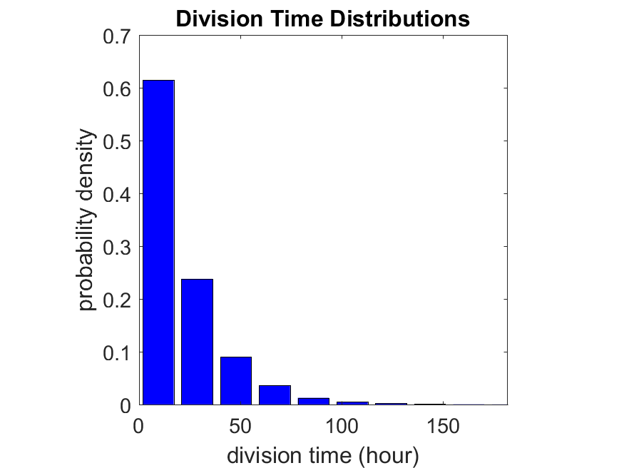
So even in this simple model, a homogeneous population of cells can show heterogeneity in their behavior. Here’s the interesting thing: let’s now give each cell its own division parameter \(r_i\) from a normal distribution with mean \(0.05 \textrm{ hr}^{-1}\) and a relative standard deviation of 25%: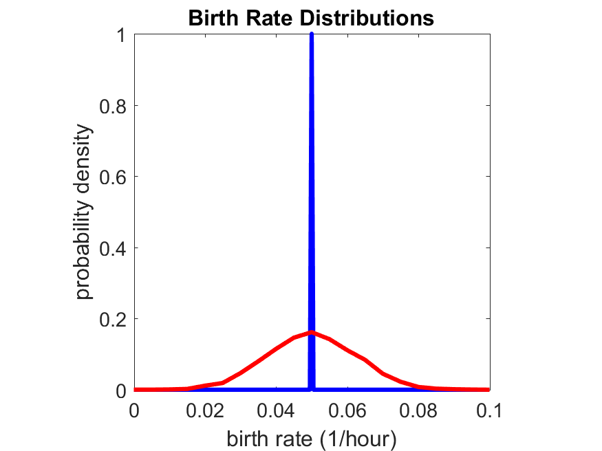
If we repeat the experiment, we get the same distribution of cell division times!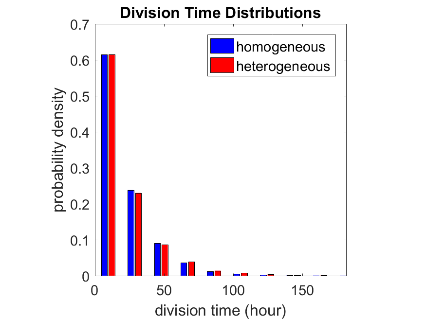
So in this case, based solely on observations of the phenotypic heterogeneity (the division times), it is impossible to distinguish a “genetically” homogeneous cell population (one with identical parameters) from a truly heterogeneous population. We would require other metrics, like tracking changes in the mean division time as cells with a higher \(r_i\) out-compete the cells with lower \(r_i\).
Lastly, I want to point out that caution is required when designing these metrics and single-cell tracking. If instead we had tracked all cells throughout the simulated experiment, including new daughter cells, and then recorded the first 10,000 cell division events, we would get a very different distribution of cell division times: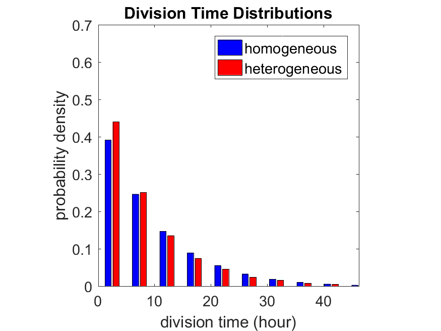
By only recording the division times for the cells that have divided, and not those that haven’t, we bias our observations towards cells with shorter division times. Indeed, the mean division time for this simulated experiment is far lower than we would expect by theory. You can try this one by running “bad_thought_experiment”.
Further reading
This post is an expansion of our recent preview in Cell Systems in Macklin (2017):
P. Macklin, When seeing isn’t believing: How math can guide our interpretation of measurements and experiments. Cell Sys., 2017 (in press). DOI: 10.1016/j.cells.2017.08.005
And the original work on apparent heterogeneity in collective cell migration is by Schumacher et al. (2017):
L. Schumacher et al., Semblance of Heterogeneity in Collective Cell Migration. Cell Sys., 2017 (in press). DOI: 10.1016/j.cels.2017.06.006
You can read some more on relating exponential distributions and Poisson processes to common discrete mathematical models of cell populations in Macklin et al. (2012):
P. Macklin, et al., Patient-calibrated agent-based modelling of ductal carcinoma in situ (DCIS): From microscopic measurements to macroscopic predictions of clinical progression. J. Theor. Biol. 301:122-40, 2012. DOI: 10.1016/j.jtbi.2012.02.002.
Lastly, I’d be delighted if you took a look at the open source software we have been developing for 3-D simulations of multicellular systems biology:
http://OpenSource.MathCancer.org
And you can always keep up-to-date by following us on Twitter: @MathCancer.
MathCancer C++ Style and Practices Guide
As PhysiCell, BioFVM, and other open source projects start to gain new users and contributors, it’s time to lay out a coding style. We have three goals here:
- Consistency: It’s easier to understand and contribute to the code if it’s written in a consistent way.
- Readability: We want the code to be as readable as possible.
- Reducing errors: We want to avoid coding styles that are more prone to errors. (e.g., code that can be broken by introducing whitespace).
So, here is the guide (revised June 2017). I expect to revise this guide from time to time.
Place braces on separate lines in functions and classes.
I find it much easier to read a class if the braces are on separate lines, with good use of whitespace. Remember: whitespace costs almost nothing, but reading and understanding (and time!) are expensive.
DON’T
class Cell{
public:
 double some_variable;
 bool some_extra_variable;

 Cell(); };

class Phenotype{
public:
 double some_variable;
 bool some_extra_variable;

 Phenotype();
};
DO:
class Cell
{
 public:
     double some_variable;
     bool some_extra_variable;

     Cell();
};

class Phenotype
{
 public:
     double some_variable;
     bool some_extra_variable;

     Phenotype();
};
Enclose all logic in braces, even when optional.
In C/C++, you can omit the curly braces in some cases. For example, this is legal
if( distance > 1.5*cell_radius )
     interaction = false;
force = 0.0; // is this part of the logic, or a separate statement?
error = false;
However, this code is ambiguous to interpret. Moreover, small changes to whitespace–or small additions to the logic–could mess things up here. Use braces to make the logic crystal clear:
DON’T
if( distance > 1.5*cell_radius )
     interaction = false;
force = 0.0; // is this part of the logic, or a separate statement?
error = false;

if( condition1 == true )
  do_something1 = true;
elseif( condition2 == true )
  do_something2 = true;
else
  do_something3 = true;
DO
if( distance > 1.5*cell_radius )
{
     interaction = false;
     force = 0.0;
}
error = false;

if( condition1 == true )
{ do_something1 = true; }
elseif( condition2 == true )
{ do_something2 = true; }
else
{ do_something3 = true; }
Put braces on separate lines in logic, except for single-line logic.
This style rule relates to the previous point, to improve readability.
DON’T
if( distance > 1.5*cell_radius ){
     interaction = false;
     force = 0.0; }

if( condition1 == true ){ do_something1 = true; }
elseif( condition2 == true ){
  do_something2 = true; }
else
{ do_something3 = true; error = true; }
DO
if( distance > 1.5*cell_radius )
{
     interaction = false;
     force = 0.0;
}

if( condition1 == true )
{ do_something1 = true; } // this is fine
elseif( condition2 == true )
{
     do_something2 = true; // this is better
}
else
{
     do_something3 = true;
     error = true;
}
See how much easier that code is to read? The logical structure is crystal clear, and adding more to the logic is simple.
End all functions with a return, even if void.
For clarity, definitively state that a function is done by using return.
DON’T
void my_function( Cell& cell )
{
     cell.phenotype.volume.total *= 2.0;
     cell.phenotype.death.rates[0] = 0.02;
     // Are we done, or did we forget something?
     // is somebody still working here?
}
DO
void my_function( Cell& cell )
{
     cell.phenotype.volume.total *= 2.0;
     cell.phenotype.death.rates[0] = 0.02;
     return;
}
Use tabs to indent the contents of a class or function.
This is to make the code easier to read. (Unfortunately PHP/HTML makes me use five spaces here instead of tabs.)
DON’T
class Secretion
{
 public:
std::vector<double> secretion_rates;
std::vector<double> uptake_rates;
std::vector<double> saturation_densities;
};

void my_function( Cell& cell )
{
cell.phenotype.volume.total *= 2.0;
cell.phenotype.death.rates[0] = 0.02;
return;
}
DO
class Secretion
{
 public:
     std::vector<double> secretion_rates;
     std::vector<double> uptake_rates;
     std::vector<double> saturation_densities;
};

void my_function( Cell& cell )
{
     cell.phenotype.volume.total *= 2.0;
     cell.phenotype.death.rates[0] = 0.02;
     return;
}
Use a single space to indent public and other keywords in a class.
This gets us some nice formatting in classes, without needing two tabs everywhere.
DON’T
class Secretion
{
public:
std::vector<double> secretion_rates;
std::vector<double> uptake_rates;
std::vector<double> saturation_densities;
}; // not enough whitespace

class Errors
{
     private:
          std::string none_of_your_business
     public:
          std::string error_message;
          int error_code;
}; // too much whitespace!
DO
class Secretion
{
 private:
 public:
     std::vector<double> secretion_rates;
     std::vector<double> uptake_rates;
     std::vector<double> saturation_densities;
};

class Errors
{
 private:
     std::string none_of_your_business
 public:
     std::string error_message;
     int error_code;
};
Avoid arcane operators, when clear logic statements will do.
It can be difficult to decipher code with statements like this:
phenotype.volume.fluid=phenotype.volume.fluid<0?0:phenotype.volume.fluid;
Moreover, C and C++ can treat precedence of ternary operators very differently, so subtle bugs can creep in when using the “fancier” compact operators. Variations in how these operators work across languages are an additional source of error for programmers switching between languages in their daily scientific workflows. Wherever possible (and unless there is a significant performance reason to do so), use clear logical structures that are easy to read even if you only dabble in C/C++. Compiler-time optimizations will most likely eliminate any performance gains from these goofy operators.
DON’T
// if the fluid volume is negative, set it to zero
phenotype.volume.fluid=phenotype.volume.fluid<0.0?0.0:pCell->phenotype.volume.fluid;
DO
if( phenotype.volume.fluid < 0.0 )
{
     phenotype.volume.fluid = 0.0;
}
Here’s the funny thing: the second logic is much clearer, and it took fewer characters, even with extra whitespace for readability!
Pass by reference where possible.
Passing by reference is a great way to boost performance: we can avoid (1) allocating new temporary memory, (2) copying data into the temporary memory, (3) passing the temporary data to the function, and (4) deallocating the temporary memory once finished.
DON’T
double some_function( Cell cell )
{
     return = cell.phenotype.volume.total + 3.0;
}
// This copies cell and all its member data!
DO
double some_function( Cell& cell )
{
     return = cell.phenotype.volume.total + 3.0;
}
// This just accesses the original cell data without recopying it.
Where possible, pass by reference instead of by pointer.
There is no performance advantage to passing by pointers over passing by reference, but the code is simpler / clearer when you can pass by reference. It makes code easier to write and understand if you can do so. (If nothing else, you save yourself character of typing each time you can replace “->” by “.”!)
DON’T
double some_function( Cell* pCell )
{
     return = pCell->phenotype.volume.total + 3.0;
}
// Writing and debugging this code can be error-prone.
DO
double some_function( Cell& cell )
{
     return = cell.phenotype.volume.total + 3.0;
}
// This is much easier to write.
Be careful with static variables. Be thread safe!
PhysiCell relies heavily on parallelization by OpenMP, and so you should write functions under the assumption that they may be executed many times simultaneously. One easy source of errors is in static variables:
DON’T
double some_function( Cell& cell )
{
     static double four_pi = 12.566370614359172;
     static double output;
     output = cell.phenotype.geometry.radius;
     output *= output;
     output *= four_pi;
     return output;
}
// If two instances of some_function are running, they will both modify
// the *same copy* of output
DO
double some_function( Cell& cell )
{
     static double four_pi = 12.566370614359172;
     double output;
     output = cell.phenotype.geometry.radius;
     output *= output;
     output *= four_pi;
     return output;
}
// If two instances of some_function are running, they will both modify
// the their own copy of output, but still use the more efficient, once-
// allocated copy of four_pi. This one is safe for OpenMP.
Use std:: instead of “using namespace std”
PhysiCell uses the BioFVM and PhysiCell namespaces to avoid potential collision with other codes. Other codes using PhysiCell may use functions that collide with the standard namespace. So, we formally use std:: whenever using functions in the standard namespace.
DON’T
using namespace std;

cout << "Hi, Mom, I learned to code today!" << endl;
string my_string = "Cheetos are good, but Doritos are better.";
cout << my_string << endl;

vector<double> my_vector;
vector.resize( 3, 0.0 );
DO
std::cout << "Hi, Mom, I learned to code today!" << std::endl;
std::string my_string = "Cheetos are good, but Doritos are better.";
std::cout << my_string << std::endl;

std::vector<double> my_vector;
my_vector.resize( 3, 0.0 );
Camelcase is ugly. Use underscores.
This is purely an aesthetic distinction, but CamelCaseCodeIsUglyAndDoYouUseDNAorDna?
DON’T
double MyVariable1;
bool ProteinsInExosomes;
int RNAtranscriptionCount;

void MyFunctionDoesSomething( Cell& ImmuneCell );
DO
double my_variable1;
bool proteins_in_exosomes;
int RNA_transcription_count;

void my_function_does_something( Cell& immune_cell );
Use capital letters to declare a class. Use lowercase for instances.
To help in readability and consistency, declare classes with capital letters (but no camelcase), and use lowercase for instances of those classes.
DON’T
class phenotype;

class cell
{
 public:
     std::vector<double> position;
     phenotype Phenotype;
};

class ImmuneCell : public cell
{
 public:
     std::vector<double> surface_receptors;
};

void do_something( cell& MyCell , ImmuneCell& immuneCell );

cell Cell;
ImmuneCell MyImmune_cell;

do_something( Cell, MyImmune_cell );
DO
class Phenotype;

class Cell
{
 public:
     std::vector<double> position;
     Phenotype phenotype;
};

class Immune_Cell : public Cell
{
 public:
     std::vector<double> surface_receptors;
};

void do_something( Cell& my_cell , Immune_Cell& immune_cell );

Cell cell;
Immune_Cell my_immune_cell;

do_something( cell, my_immune_cell );
DCIS modeling paper accepted
I am pleased to report that our paper has now been accepted. You can download the accepted preprint here. We also have a lot of supplementary material, including simulation movies, simulation datasets (for 0, 15, 30, adn 45 days of growth), and open source C++ code for postprocessing and visualization.
I discussed the results in detail here, but here’s the short version:
- We use a mechanistic, agent-based model of individual cancer cells growing in a duct. Cells are moved by adhesive and repulsive forces exchanged with other cells and the basement membrane. Cell phenotype is controlled by stochastic processes.
- We constrained all parameter expected to be relatively independent of patients by a careful analysis of the experimental biological and clinical literature.
- We developed the very first patient-specific calibration method, using clinically-accessible pathology. This is a key point in future patient-tailored predictions and surgical/therapeutic planning.
- The model made numerous quantitative predictions, such as:
- The tumor grows at a constant rate, between 7 to 10 mm/year. This is right in the middle of the range reported in the clinic.
- The tumor’s size in mammgraphy is linearly correlated with the post-surgical pathology size. When we linearly extrapolate our correlation across two orders of magnitude, it goes right through the middle of a cluster of 87 clinical data points.
- The tumor necrotic core has an age structuring: with oldest, calcified material in the center, and newest, most intact necrotic cells at the outer edge.
- The appearance of a “typical” DCIS duct cross-section varies with distance from the leading edge; all types of cross-sections predicted by our model are observed in patient pathology.
- The model also gave new insight on the underlying biology of breast cancer, such as:
- The split between the viable rim and necrotic core (observed almost universally in pathology) is not just an artifact, but an actual biomechanical effect from fast necrotic cell lysis.
- The constant rate of tumor growth arises from the biomechanical stress relief provided by lysing necrotic cells. This points to the critical role of intracellular and intra-tumoral water transport in determining the qualitative and quantitative behavior of tumors.
- Pyknosis (nuclear degradation in necrotic cells), must occur at a time scale between that of cell lysis (on the order of hours) and cell calcification (on the order of weeks).
- The current model cannot explain the full spectrum of calcification types; other biophysics, such as degradation over a long, 1-2 month time scale, must be at play.
Now hiring: Postdoctoral Researcher
I just posted a job opportunity for a postdoctoral researcher for computational modeling of breast, prostate, and metastatic cancer, with a heavy emphasis on calibrating (and validating!) to in vitro, in vivo, and clinical data.
If you’re a talented computational modeler and have a passion for applying mathematics to make a difference in clinical care, please read the job posting and apply!
(Note: Interested students in the Los Angeles/Orange County area may want to attend my applied math seminar talk at UCI next week to learn more about this work.)
MMCL welcomes Gianluca D’Antonio
The Macklin Math Cancer Lab is pleased to welcome Gianluca D’Antonio, a M.S. student of Luigi Preziosi and mathematician from Politecnico di Torino. Gianluca, who brings with him a wealth of expertise in biomechanics modeling, will spend 6 months at CAMM at the Keck School of Medicine of USC to model basement membrane deformation by growing tumors, biomechanical feedback between the stroma and growing tumors, and related problems. Gianluca’s interests and expertise fit very nicely into our broader vision of mechanistic cancer modeling, as well as USC / CAMM’s focus on applying the physical sciences to cancer (as part of the USC-led PSOC).
He is our first international visiting scholar, and we’re very excited for the multidisciplinary work we will accomplish together! So, please join us in welcoming Gianluca!