Category: heterogeneity
A small computational thought experiment
In Macklin (2017), I briefly touched on a simple computational thought experiment that shows that for a group of homogeneous cells, you can observe substantial heterogeneity in cell behavior. This “thought experiment” is part of a broader preview and discussion of a fantastic paper by Linus Schumacher, Ruth Baker, and Philip Maini published in Cell Systems, where they showed that a migrating collective homogeneous cells can show heterogeneous behavior when quantitated with new migration metrics. I highly encourage you to check out their work!
In this blog post, we work through my simple thought experiment in a little more detail.
Note: If you want to reference this blog post, please cite the Cell Systems preview article:
P. Macklin, When seeing isn’t believing: How math can guide our interpretation of measurements and experiments. Cell Sys., 2017 (in press). DOI: 10.1016/j.cells.2017.08.005
The thought experiment
Consider a simple (and widespread) model of a population of cycling cells: each virtual cell (with index i) has a single “oncogene” \( r_i \) that sets the rate of progression through the cycle. Between now (t) and a small time from now ( \(t+\Delta t\)), the virtual cell has a probability \(r_i \Delta t\) of dividing into two daughter cells. At the population scale, the overall population growth model that emerges from this simple single-cell model is:
\[\frac{dN}{dt} = \langle r\rangle N, \]
where \( \langle r \rangle \) the mean division rate over the cell population, and N is the number of cells. See the discussion in the supplementary information for Macklin et al. (2012).
Now, suppose (as our thought experiment) that we could track individual cells in the population and track how long it takes them to divide. (We’ll call this the division time.) What would the distribution of cell division times look like, and how would it vary with the distribution of the single-cell rates \(r_i\)?
Mathematical method
In the Matlab script below, we implement this cell cycle model as just about every discrete model does. Here’s the pseudocode:
t = 0;
while( t < t_max )
    for i=1:Cells.size()
        u = random_number();
        if( u < Cells[i].birth_rate * dt )
            Cells[i].division_time = Cells[i].age;
            Cells[i].divide();
        end
    end
    t = t+dt;
end
That is, until we’ve reached the final simulation time, loop through all the cells and decide if they should divide: For each cell, choose a random number between 0 and 1, and if it’s smaller than the cell’s division probability (\(r_i \Delta t\)), then divide the cell and write down the division time.
As an important note, we have to track the same cells until they all divide, rather than merely record which cells have divided up to the end of the simulation. Otherwise, we end up with an observational bias that throws off our recording. See more below.
The sample code
You can download the Matlab code for this example at:
http://MathCancer.org/files/matlab/thought_experiment_matlab(Macklin_Cell_Systems_2017).zip
Extract all the files, and run “thought_experiment” in Matlab (or Octave, if you don’t have a Matlab license or prefer an open source platform) for the main result.
All these Matlab files are available as open source, under the GPL license (version 3 or later).
Results and discussion
First, let’s see what happens if all the cells are identical, with \(r = 0.05 \textrm{ hr}^{-1}\). We run the script, and track the time for each of 10,000 cells to divide. As expected by theory (Macklin et al., 2012) (but perhaps still a surprise if you haven’t looked), we get an exponential distribution of division times, with mean time \(1/\langle r \rangle\):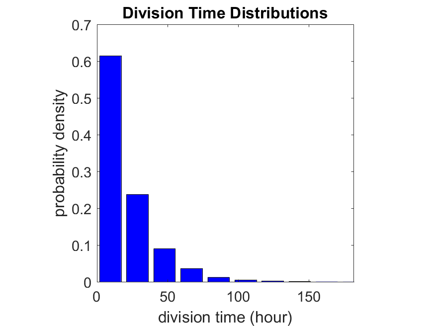
So even in this simple model, a homogeneous population of cells can show heterogeneity in their behavior. Here’s the interesting thing: let’s now give each cell its own division parameter \(r_i\) from a normal distribution with mean \(0.05 \textrm{ hr}^{-1}\) and a relative standard deviation of 25%: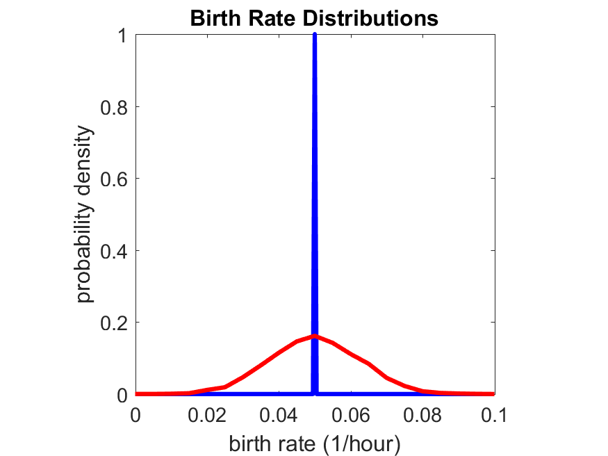
If we repeat the experiment, we get the same distribution of cell division times!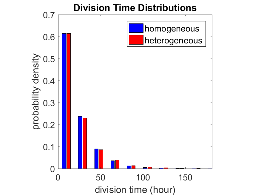
So in this case, based solely on observations of the phenotypic heterogeneity (the division times), it is impossible to distinguish a “genetically” homogeneous cell population (one with identical parameters) from a truly heterogeneous population. We would require other metrics, like tracking changes in the mean division time as cells with a higher \(r_i\) out-compete the cells with lower \(r_i\).
Lastly, I want to point out that caution is required when designing these metrics and single-cell tracking. If instead we had tracked all cells throughout the simulated experiment, including new daughter cells, and then recorded the first 10,000 cell division events, we would get a very different distribution of cell division times: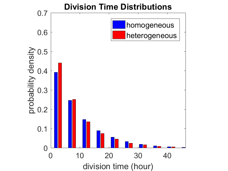
By only recording the division times for the cells that have divided, and not those that haven’t, we bias our observations towards cells with shorter division times. Indeed, the mean division time for this simulated experiment is far lower than we would expect by theory. You can try this one by running “bad_thought_experiment”.
Further reading
This post is an expansion of our recent preview in Cell Systems in Macklin (2017):
P. Macklin, When seeing isn’t believing: How math can guide our interpretation of measurements and experiments. Cell Sys., 2017 (in press). DOI: 10.1016/j.cells.2017.08.005
And the original work on apparent heterogeneity in collective cell migration is by Schumacher et al. (2017):
L. Schumacher et al., Semblance of Heterogeneity in Collective Cell Migration. Cell Sys., 2017 (in press). DOI: 10.1016/j.cels.2017.06.006
You can read some more on relating exponential distributions and Poisson processes to common discrete mathematical models of cell populations in Macklin et al. (2012):
P. Macklin, et al., Patient-calibrated agent-based modelling of ductal carcinoma in situ (DCIS): From microscopic measurements to macroscopic predictions of clinical progression. J. Theor. Biol. 301:122-40, 2012. DOI: 10.1016/j.jtbi.2012.02.002.
Lastly, I’d be delighted if you took a look at the open source software we have been developing for 3-D simulations of multicellular systems biology:
http://OpenSource.MathCancer.org
And you can always keep up-to-date by following us on Twitter: @MathCancer.