Category: cancer modeling
A small computational thought experiment
In Macklin (2017), I briefly touched on a simple computational thought experiment that shows that for a group of homogeneous cells, you can observe substantial heterogeneity in cell behavior. This “thought experiment” is part of a broader preview and discussion of a fantastic paper by Linus Schumacher, Ruth Baker, and Philip Maini published in Cell Systems, where they showed that a migrating collective homogeneous cells can show heterogeneous behavior when quantitated with new migration metrics. I highly encourage you to check out their work!
In this blog post, we work through my simple thought experiment in a little more detail.
Note: If you want to reference this blog post, please cite the Cell Systems preview article:
P. Macklin, When seeing isn’t believing: How math can guide our interpretation of measurements and experiments. Cell Sys., 2017 (in press). DOI: 10.1016/j.cells.2017.08.005
The thought experiment
Consider a simple (and widespread) model of a population of cycling cells: each virtual cell (with index i) has a single “oncogene” \( r_i \) that sets the rate of progression through the cycle. Between now (t) and a small time from now ( \(t+\Delta t\)), the virtual cell has a probability \(r_i \Delta t\) of dividing into two daughter cells. At the population scale, the overall population growth model that emerges from this simple single-cell model is:
\[\frac{dN}{dt} = \langle r\rangle N, \]
where \( \langle r \rangle \) the mean division rate over the cell population, and N is the number of cells. See the discussion in the supplementary information for Macklin et al. (2012).
Now, suppose (as our thought experiment) that we could track individual cells in the population and track how long it takes them to divide. (We’ll call this the division time.) What would the distribution of cell division times look like, and how would it vary with the distribution of the single-cell rates \(r_i\)?
Mathematical method
In the Matlab script below, we implement this cell cycle model as just about every discrete model does. Here’s the pseudocode:
t = 0;
while( t < t_max )
    for i=1:Cells.size()
        u = random_number();
        if( u < Cells[i].birth_rate * dt )
            Cells[i].division_time = Cells[i].age;
            Cells[i].divide();
        end
    end
    t = t+dt;
end
That is, until we’ve reached the final simulation time, loop through all the cells and decide if they should divide: For each cell, choose a random number between 0 and 1, and if it’s smaller than the cell’s division probability (\(r_i \Delta t\)), then divide the cell and write down the division time.
As an important note, we have to track the same cells until they all divide, rather than merely record which cells have divided up to the end of the simulation. Otherwise, we end up with an observational bias that throws off our recording. See more below.
The sample code
You can download the Matlab code for this example at:
http://MathCancer.org/files/matlab/thought_experiment_matlab(Macklin_Cell_Systems_2017).zip
Extract all the files, and run “thought_experiment” in Matlab (or Octave, if you don’t have a Matlab license or prefer an open source platform) for the main result.
All these Matlab files are available as open source, under the GPL license (version 3 or later).
Results and discussion
First, let’s see what happens if all the cells are identical, with \(r = 0.05 \textrm{ hr}^{-1}\). We run the script, and track the time for each of 10,000 cells to divide. As expected by theory (Macklin et al., 2012) (but perhaps still a surprise if you haven’t looked), we get an exponential distribution of division times, with mean time \(1/\langle r \rangle\):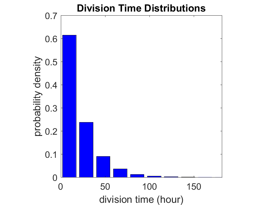
So even in this simple model, a homogeneous population of cells can show heterogeneity in their behavior. Here’s the interesting thing: let’s now give each cell its own division parameter \(r_i\) from a normal distribution with mean \(0.05 \textrm{ hr}^{-1}\) and a relative standard deviation of 25%: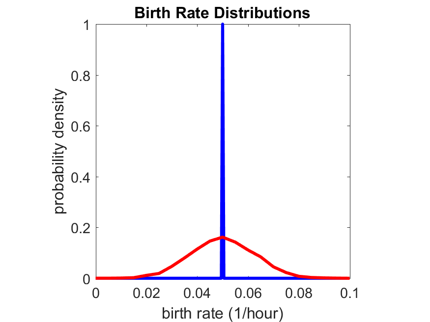
If we repeat the experiment, we get the same distribution of cell division times!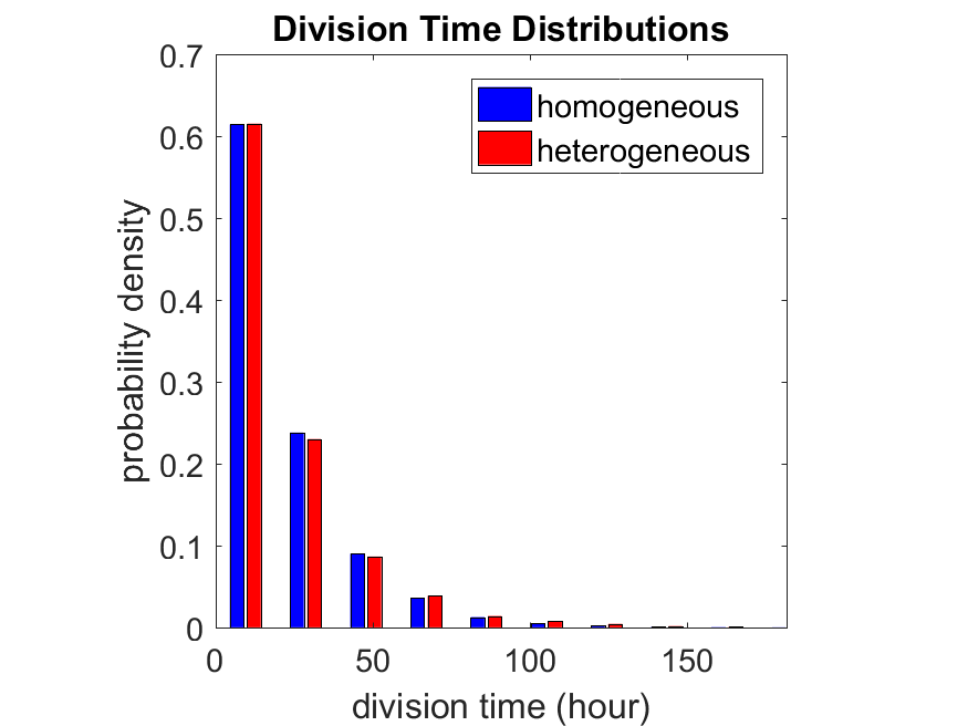
So in this case, based solely on observations of the phenotypic heterogeneity (the division times), it is impossible to distinguish a “genetically” homogeneous cell population (one with identical parameters) from a truly heterogeneous population. We would require other metrics, like tracking changes in the mean division time as cells with a higher \(r_i\) out-compete the cells with lower \(r_i\).
Lastly, I want to point out that caution is required when designing these metrics and single-cell tracking. If instead we had tracked all cells throughout the simulated experiment, including new daughter cells, and then recorded the first 10,000 cell division events, we would get a very different distribution of cell division times: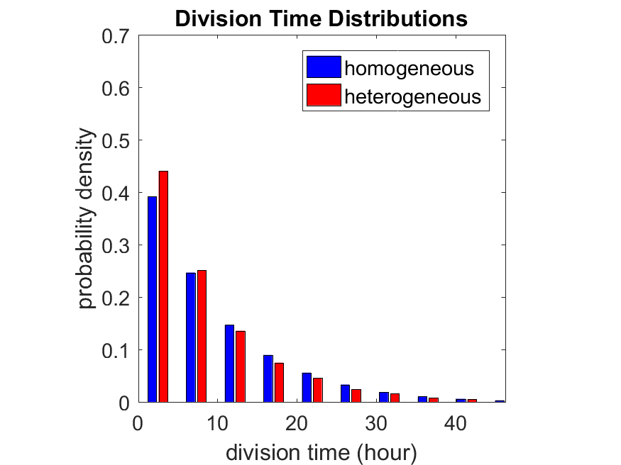
By only recording the division times for the cells that have divided, and not those that haven’t, we bias our observations towards cells with shorter division times. Indeed, the mean division time for this simulated experiment is far lower than we would expect by theory. You can try this one by running “bad_thought_experiment”.
Further reading
This post is an expansion of our recent preview in Cell Systems in Macklin (2017):
P. Macklin, When seeing isn’t believing: How math can guide our interpretation of measurements and experiments. Cell Sys., 2017 (in press). DOI: 10.1016/j.cells.2017.08.005
And the original work on apparent heterogeneity in collective cell migration is by Schumacher et al. (2017):
L. Schumacher et al., Semblance of Heterogeneity in Collective Cell Migration. Cell Sys., 2017 (in press). DOI: 10.1016/j.cels.2017.06.006
You can read some more on relating exponential distributions and Poisson processes to common discrete mathematical models of cell populations in Macklin et al. (2012):
P. Macklin, et al., Patient-calibrated agent-based modelling of ductal carcinoma in situ (DCIS): From microscopic measurements to macroscopic predictions of clinical progression. J. Theor. Biol. 301:122-40, 2012. DOI: 10.1016/j.jtbi.2012.02.002.
Lastly, I’d be delighted if you took a look at the open source software we have been developing for 3-D simulations of multicellular systems biology:
http://OpenSource.MathCancer.org
And you can always keep up-to-date by following us on Twitter: @MathCancer.
Building a Cellular Automaton Model Using BioFVM
Note: This is part of a series of “how-to” blog posts to help new users and developers of BioFVM. See below for guides to setting up a C++ compiler in Windows or OSX.
What you’ll need
- A working C++ development environment with support for OpenMP. See these prior tutorials if you need help.
- A download of BioFVM, available at http://BioFVM.MathCancer.org and http://BioFVM.sf.net. Use Version 1.1.4 or later.
- The source code for this project (see below).
Matlab or Octave for visualization. Matlab might be available for free at your university. Octave is open source and available from a variety of sources.
Our modeling task
We will implement a basic 3-D cellular automaton model of tumor growth in a well-mixed fluid, containing oxygen pO2 (mmHg) and a drug c (e.g., doxorubicin, μM), inspired by modeling by Alexander Anderson, Heiko Enderling, Jan Poleszczuk, Gibin Powathil, and others. (I highly suggest seeking out the sophisticated cellular automaton models at Moffitt’s Integrated Mathematical Oncology program!) This example shows you how to extend BioFVM into a new cellular automaton model. I’ll write a similar post on how to add BioFVM into an existing cellular automaton model, which you may already have available.
Tumor growth will be driven by oxygen availability. Tumor cells can be live, apoptotic (going through energy-dependent cell death, or necrotic (undergoing death from energy collapse). Drug exposure can both trigger apoptosis and inhibit cell cycling. We will model this as growth into a well-mixed fluid, with pO2 = 38 mmHg (about 5% oxygen: a physioxic value) and c = 5 μM.
Mathematical model
As a cellular automaton model, we will divide 3-D space into a regular lattice of voxels, with length, width, and height of 15 μm. (A typical breast cancer cell has radius around 9-10 μm, giving a typical volume around 3.6×103 μm3. If we make each lattice site have the volume of one cell, this gives an edge length around 15 μm.)
In voxels unoccupied by cells, we approximate a well-mixed fluid with Dirichlet nodes, setting pO2 = 38 mmHg, and initially setting c = 0. Whenever a cell dies, we replace it with an empty automaton, with no Dirichlet node. Oxygen and drug follow the typical diffusion-reaction equations:
\[ \frac{ \partial \textrm{pO}_2 }{\partial t} = D_\textrm{oxy} \nabla^2 \textrm{pO}_2 – \lambda_\textrm{oxy} \textrm{pO}_2 – \sum_{ \textrm{cells} i} U_{i,\textrm{oxy}} \textrm{pO}_2 \]
\[ \frac{ \partial c}{ \partial t } = D_c \nabla^2 c – \lambda_c c – \sum_{\textrm{cells }i} U_{i,c} c \]
where each uptake rate is applied across the cell’s volume. We start the treatment by setting c = 5 μM on all Dirichlet nodes at t = 504 hours (21 days). For simplicity, we do not model drug degradation (pharmacokinetics), to approximate the in vitro conditions.
In any time interval [t,t+Δt], each live tumor cell i has a probability pi,D of attempting division, probability pi,A of apoptotic death, and probability pi,N of necrotic death. (For simplicity, we ignore motility in this version.) We relate these to the birth rate bi, apoptotic death rate di,A, and necrotic death rate di,N by the linearized equations (from Macklin et al. 2012):
\[ \textrm{Prob} \Bigl( \textrm{cell } i \textrm{ becomes apoptotic in } [t,t+\Delta t] \Bigr) = 1 – \textrm{exp}\Bigl( -d_{i,A}(t) \Delta t\Bigr) \approx d_{i,A}\Delta t \]
\[ \textrm{Prob} \Bigl( \textrm{cell } i \textrm{ attempts division in } [t,t+\Delta t] \Bigr) = 1 – \textrm{exp}\Bigl( -b_i(t) \Delta t\Bigr) \approx b_{i}\Delta t \]
\[ \textrm{Prob} \Bigl( \textrm{cell } i \textrm{ becomes necrotic in } [t,t+\Delta t] \Bigr) = 1 – \textrm{exp}\Bigl( -d_{i,N}(t) \Delta t\Bigr) \approx d_{i,N}\Delta t \]
\[ \textrm{Prob} \Bigl( \textrm{dead cell } i \textrm{ lyses in } [t,t+\Delta t] \Bigr) = 1 – \textrm{exp}\Bigl( -\frac{1}{T_{i,D}} \Delta t\Bigr) \approx \frac{ \Delta t}{T_{i,D}} \]
(Illustrative) parameter values
We use Doxy = 105 μm2/min (Ghaffarizadeh et al. 2016), and we set Ui,oxy = 20 min-1 (to give an oxygen diffusion length scale of about 70 μm, with steeper gradients than our typical 100 μm length scale). We set λoxy = 0.01 min-1 for a 1 mm diffusion length scale in fluid.
We set Dc = 300 μm2/min, and Uc = 7.2×10⁻³ min-1 (Dc from Weinberg et al. (2007), and Ui,c twice as large as the reference value in Weinberg et al. (2007) to get a smaller diffusion length scale of about 204 μm). We set λc = 3.6×10⁻⁵ min-1 to give a drug diffusion length scale of about 2.9 mm in fluid.
We use TD = 8.6 hours for apoptotic cells, and TD = 60 days for necrotic cells (Macklin et al., 2013). However, note that necrotic and apoptotic cells lose volume quickly, so one may want to revise those time scales to match the point where a cell loses 90% of its volume.
Functional forms for the birth and death rates
We model pharmacodynamics with an area-under-the-curve (AUC) type formulation. If c(t) is the drug concentration at any cell i‘s location at time t, then let its integrated exposure Ei(t) be
\[ E_i(t) = \int_0^t c(s) \: ds \]
and we model its response with a Hill function
\[ R_i(t) = \frac{ E_i^h(t) }{ \alpha_i^h + E_i^h(t) }, \]
where h is the drug’s Hill exponent for the cell line, and α is the exposure for a half-maximum effect.
We model the microenvironment-dependent birth rate by:
\[ b_i(t) = \left\{ \begin{array}{lr} b_{i,P} \left( 1 – \eta_i R_i(t) \right) & \textrm{ if } \textrm{pO}_{2,P} < \textrm{pO}_2 \\ \\ b_{i,P} \left( \frac{\textrm{pO}_{2}-\textrm{pO}_{2,N}}{\textrm{pO}_{2,P}-\textrm{pO}_{2,N}}\right) \Bigl( 1 – \eta_i R_i(t) \Bigr) & \textrm{ if } \textrm{pO}_{2,N} < \textrm{pO}_2 \le \textrm{pO}_{2,P} \\ \\ 0 & \textrm{ if } \textrm{pO}_2 \le \textrm{pO}_{2,N}\end{array} \right. \]
where pO2,P is the physioxic oxygen value (38 mmHg), and pO2,N is a necrotic threshold (we use 5 mmHg), and 0 < η < 1 the drug’s birth inhibition. (A fully cytostatic drug has η = 1.)
We model the microenvironment-dependent apoptosis rate by:
\[ d_{i,A}(t) = d_{i,A}^* + \Bigl( d_{i,A}^\textrm{max} – d_{i,A}^* \Bigr) R_i(t) \]
\[ d_{i,N}(t) = \left\{ \begin{array}{lr} 0 & \textrm{ if } \textrm{pO}_{2,N} < \textrm{pO}_{2} \\ \\ d_{i,N}^* & \textrm{ if } \textrm{pO}_{2} \le \textrm{pO}_{2,N} \end{array}\right. \]
(Illustrative) parameter values
We use bi,P = 0.05 hour-1 (for a 20 hour cell cycle in physioxic conditions), di,A* = 0.01 bi,P, and di,N* = 0.04 hour-1 (so necrotic cells survive around 25 hours in low oxygen conditions).
We set α = 30 μM*hour (so that cells reach half max response after 6 hours’ exposure at a maximum concentration c = 5 μM), h = 2 (for a smooth effect), η = 0.25 (so that the drug is partly cytostatic), and di,Amax = 0.1 hour^-1 (so that cells survive about 10 hours after reaching maximum response).
Building the Cellular Automaton Model in BioFVM
BioFVM already includes Basic_Agents for cell-based substrate sources and sinks. We can extend these basic agents into full-fledged automata, and then arrange them in a lattice to create a full cellular automata model. Let’s sketch that out now.
Extending Basic_Agents to Automata
The main idea here is to define an Automaton class which extends (and therefore includes) the Basic_Agent class. This will give each Automaton full access to the microenvironment defined in BioFVM, including the ability to secrete and uptake substrates. We also make sure each Automaton “knows” which microenvironment it lives in (contains a pointer pMicroenvironment), and “knows” where it lives in the cellular automaton lattice. (More on that in the following paragraphs.)
So, as a schematic (just sketching out the most important members of the class):
class Standard_Data; // define per-cell biological data, such as phenotype,
	// cell cycle status, etc..
class Custom_Data; // user-defined custom data, specific to a model.

class Automaton : public Basic_Agent
{
	private:
		Microenvironment* pMicroenvironment;

		CA_Mesh* pCA_mesh;
		int voxel_index;

	protected:
	public:
		// neighbor connectivity information
		std::vector<Automaton*> neighbors;
		std::vector<double> neighbor_weights;

		Standard_Data standard_data;
		void (*current_state_rule)( Automaton& A , double );

		Automaton();
		void copy_parameters( Standard_Data& SD  );
		void overwrite_from_automaton( Automaton& A );

		void set_cellular_automaton_mesh( CA_Mesh* pMesh );
		CA_Mesh* get_cellular_automaton_mesh( void ) const;

		void set_voxel_index( int );
		int get_voxel_index( void ) const;

		void set_microenvironment( Microenvironment* pME );
		Microenvironment* get_microenvironment( void );

		// standard state changes
		bool attempt_division( void );
		void become_apoptotic( void );
		void become_necrotic( void );
		void perform_lysis( void );

		// things the user needs to define

		Custom_Data custom_data;

		// use this rule to add custom logic
		void (*custom_rule)( Automaton& A , double);
};
So, the Automaton class includes everything in the Basic_Agent class, some Standard_Data (things like the cell state and phenotype, and per-cell settings), (user-defined) Custom_Data, basic cell behaviors like attempting division into an empty neighbor lattice site, and user-defined custom logic that can be applied to any automaton. To avoid lots of switch/case and if/then logic, each Automaton has a function pointer for its current activity (current_state_rule), which can be overwritten any time.
Each Automaton also has a list of neighbor Automata (their memory addresses), and weights for each of these neighbors. Thus, you can distance-weight the neighbors (so that corner elements are farther away), and very generalized neighbor models are possible (e.g., all lattice sites within a certain distance). When updating a cellular automaton model, such as to kill a cell, divide it, or move it, you leave the neighbor information alone, and copy/edit the information (standard_data, custom_data, current_state_rule, custom_rule). In many ways, an Automaton is just a bucket with a cell’s information in it.
Note that each Automaton also “knows” where it lives (pMicroenvironment and voxel_index), and knows what CA_Mesh it is attached to (more below).
Connecting Automata into a Lattice
An automaton by itself is lost in the world–it needs to link up into a lattice organization. Here’s where we define a CA_Mesh class, to hold the entire collection of Automata, setup functions (to match to the microenvironment), and two fundamental operations at the mesh level: copying automata (for cell division), and swapping them (for motility). We have provided two functions to accomplish these tasks, while automatically keeping the indexing and BioFVM functions correctly in sync. Here’s what it looks like:
class CA_Mesh{
	private:
		Microenvironment* pMicroenvironment;
		Cartesian_Mesh* pMesh;

		std::vector<Automaton> automata;
		std::vector<int> iteration_order;
	protected:
	public:
		CA_Mesh();

		// setup to match a supplied microenvironment
		void setup( Microenvironment& M );
		// setup to match the default microenvironment
		void setup( void );

		int number_of_automata( void ) const;

		void randomize_iteration_order( void );

		void swap_automata( int i, int j );
		void overwrite_automaton( int source_i, int destination_i );

		// return the automaton sitting in the ith lattice site
		Automaton& operator[]( int i );

		// go through all nodes according to random shuffled order
		void update_automata( double dt );
};
So, the CA_Mesh has a vector of Automata (which are never themselves moved), pointers to the microenvironment and its mesh, and a vector of automata indices that gives the iteration order (so that we can sample the automata in a random order). You can easily access an automaton with operator[], and copy the data from one Automaton to another with overwrite_automaton() (e.g, for cell division), and swap two Automata’s data (e.g., for cell migration) with swap_automata(). Finally, calling update_automata(dt) iterates through all the automata according to iteration_order, calls their current_state_rules and custom_rules, and advances the automata by dt.
Interfacing Automata with the BioFVM Microenvironment
The setup function ensures that the CA_Mesh is the same size as the Microenvironment.mesh, with same indexing, and that all automata have the correct volume, and dimension of uptake/secretion rates and parameters. If you declare and set up the Microenvironment first, all this is take care of just by declaring a CA_Mesh, as it seeks out the default microenvironment and sizes itself accordingly:
// declare a microenvironment
Microenvironment M;
// do things to set it up -- see prior tutorials
// declare a Cellular_Automaton_Mesh
CA_Mesh CA_model;
// it's already good to go, initialized to empty automata:
CA_model.display();
If you for some reason declare the CA_Mesh fist, you can set it up against the microenvironment:
// declare a CA_Mesh
CA_Mesh CA_model;
// declare a microenvironment
Microenvironment M;
// do things to set it up -- see prior tutorials
// initialize the CA_Mesh to match the microenvironment
CA_model.setup( M );
// it's already good to go, initialized to empty automata:
CA_model.display();
Because each Automaton is in the microenvironment and inherits functions from Basic_Agent, it can secrete or uptake. For example, we can use functions like this one:
void set_uptake( Automaton& A, std::vector<double>& uptake_rates )
{
extern double BioFVM_CA_diffusion_dt;
// update the uptake_rates in the standard_data
A.standard_data.uptake_rates = uptake_rates;
// now, transfer them to the underlying Basic_Agent
*(A.uptake_rates) = A.standard_data.uptake_rates;
// and make sure the internal constants are self-consistent
A.set_internal_uptake_constants( BioFVM_CA_diffusion_dt );
}
A function acting on an automaton can sample the microenvironment to change parameters and state. For example:
void do_nothing( Automaton& A, double dt )
{ return; }

void microenvironment_based_rule( Automaton& A, double dt )
{
	// sample the microenvironment
	std::vector<double> MS = (*A.get_microenvironment())( A.get_voxel_index() );

	// if pO2 < 5 mmHg, set the cell to a necrotic state
	if( MS[0] < 5.0 ) { A.become_necrotic(); } // if drug > 5 uM, set the birth rate to zero
	if( MS[1] > 5 )
	{ A.standard_data.birth_rate = 0.0; }

	// set the custom rule to something else
	A.custom_rule = do_nothing;

	return;
}
Implementing the mathematical model in this framework
We give each tumor cell a tumor_cell_rule (using this for custom_rule):
void viable_tumor_rule( Automaton& A, double dt )
{
	// If there's no cell here, don't bother.
	if( A.standard_data.state_code == BioFVM_CA_empty )
	{ return; }

	// sample the microenvironment
	std::vector<double> MS = (*A.get_microenvironment())( A.get_voxel_index() );

	// integrate drug exposure
	A.standard_data.integrated_drug_exposure += ( MS[1]*dt );
	A.standard_data.drug_response_function_value = pow( A.standard_data.integrated_drug_exposure,
		A.standard_data.drug_hill_exponent );
	double temp = pow( A.standard_data.drug_half_max_drug_exposure,
		A.standard_data.drug_hill_exponent );
	temp += A.standard_data.drug_response_function_value;
	A.standard_data.drug_response_function_value /= temp;

	// update birth rates (which themselves update probabilities)
	update_birth_rate( A, MS, dt );
	update_apoptotic_death_rate( A, MS, dt );
	update_necrotic_death_rate( A, MS, dt );

	return;
}
The functional tumor birth and death rates are implemented as:
void update_birth_rate( Automaton& A, std::vector<double>& MS, double dt )
{
	static double O2_denominator = BioFVM_CA_physioxic_O2 - BioFVM_CA_necrotic_O2;

	A.standard_data.birth_rate = 	A.standard_data.drug_response_function_value;
		// response
	A.standard_data.birth_rate *= A.standard_data.drug_max_birth_inhibition;
		// inhibition*response;
	A.standard_data.birth_rate *= -1.0;
		// - inhibition*response
	A.standard_data.birth_rate += 1.0;
		// 1 - inhibition*response
	A.standard_data.birth_rate *= viable_tumor_cell.birth_rate;
		// birth_rate0*(1 - inhibition*response)

	double temp1 = MS[0] ; // O2
	temp1 -= BioFVM_CA_necrotic_O2;
	temp1 /= O2_denominator;

	A.standard_data.birth_rate *= temp1;
	if( A.standard_data.birth_rate < 0 )
	{ A.standard_data.birth_rate = 0.0; }

	A.standard_data.probability_of_division = A.standard_data.birth_rate;
	A.standard_data.probability_of_division *= dt;
		// dt*birth_rate*(1 - inhibition*repsonse) // linearized probability
	return;
}

void update_apoptotic_death_rate( Automaton& A, std::vector<double>& MS, double dt )
{
	A.standard_data.apoptotic_death_rate = A.standard_data.drug_max_death_rate;
		// max_rate
	A.standard_data.apoptotic_death_rate -= viable_tumor_cell.apoptotic_death_rate;
		// max_rate - background_rate
	A.standard_data.apoptotic_death_rate *= A.standard_data.drug_response_function_value;
		// (max_rate-background_rate)*response
	A.standard_data.apoptotic_death_rate += viable_tumor_cell.apoptotic_death_rate;
		// background_rate + (max_rate-background_rate)*response

	A.standard_data.probability_of_apoptotic_death = A.standard_data.apoptotic_death_rate;
	A.standard_data.probability_of_apoptotic_death *= dt;
		// dt*( background_rate + (max_rate-background_rate)*response ) // linearized probability
	return;
}

void update_necrotic_death_rate( Automaton& A, std::vector<double>& MS, double dt )
{
	A.standard_data.necrotic_death_rate = 0.0;
	A.standard_data.probability_of_necrotic_death = 0.0;

	if( MS[0] > BioFVM_CA_necrotic_O2 )
	{ return; }

	A.standard_data.necrotic_death_rate = perinecrotic_tumor_cell.necrotic_death_rate;
	A.standard_data.probability_of_necrotic_death = A.standard_data.necrotic_death_rate;
	A.standard_data.probability_of_necrotic_death *= dt;
		// dt*necrotic_death_rate

	return;
}
And each fluid voxel (Dirichlet nodes) is implemented as the following (to turn on therapy at 21 days):
void fluid_rule( Automaton& A, double dt )
{
	static double activation_time = 504;
	static double activation_dose = 5.0;
	static std::vector<double> activated_dirichlet( 2 , BioFVM_CA_physioxic_O2 );
	static bool initialized = false;
	if( !initialized )
	{
		activated_dirichlet[1] = activation_dose;
		initialized = true;
	}

	if( fabs( BioFVM_CA_elapsed_time - activation_time ) < 0.01 ) { int ind = A.get_voxel_index(); if( A.get_microenvironment()->mesh.voxels[ind].is_Dirichlet )
		{
			A.get_microenvironment()->update_dirichlet_node( ind, activated_dirichlet );
		}
	}
}
At the start of the simulation, each non-cell automaton has its custom_rule set to fluid_rule, and each tumor cell Automaton has its custom_rule set to viable_tumor_rule. Here’s how:
void setup_cellular_automata_model( Microenvironment& M, CA_Mesh& CAM )
{
	// Fill in this environment
	double tumor_radius = 150;
	double tumor_radius_squared = tumor_radius * tumor_radius;

	std::vector<double> tumor_center( 3, 0.0 );

	std::vector<double> dirichlet_value( 2 , 1.0 );
	dirichlet_value[0] = 38; //physioxia
	dirichlet_value[1] = 0; // drug

	for( int i=0 ; i < M.number_of_voxels() ;i++ )
	{
		std::vector<double> displacement( 3, 0.0 );
		displacement = M.mesh.voxels[i].center;
		displacement -= tumor_center;
		double r2 = norm_squared( displacement );

		if( r2 > tumor_radius_squared ) // well_mixed_fluid
		{
			M.add_dirichlet_node( i, dirichlet_value );
			CAM[i].copy_parameters( well_mixed_fluid );
			CAM[i].custom_rule = fluid_rule;
			CAM[i].current_state_rule = do_nothing;
		}
		else // tumor
		{
			CAM[i].copy_parameters( viable_tumor_cell );
			CAM[i].custom_rule = viable_tumor_rule;
			CAM[i].current_state_rule = advance_live_state;
		}

	}
}
Overall program loop
There are two inherent time scales in this problem: cell processes like division and death (happen on the scale of hours), and transport (happens on the order of minutes). We take advantage of this by defining two step sizes:
double BioFVM_CA_dt = 3;
std::string BioFVM_CA_time_units = "hr";
double BioFVM_CA_save_interval = 12;
double BioFVM_CA_max_time = 24*28;
double BioFVM_CA_elapsed_time = 0.0;

double BioFVM_CA_diffusion_dt = 0.05;

std::string BioFVM_CA_transport_time_units = "min";
double BioFVM_CA_diffusion_max_time = 5.0;
Every time the simulation advances by BioFVM_CA_dt (on the order of hours), we run diffusion to quasi-steady state (for BioFVM_CA_diffusion_max_time, on the order of minutes), using time steps of size BioFVM_CA_diffusion time. We performed numerical stability and convergence analyses to determine 0.05 min works pretty well for regular lattice arrangements of cells, but you should always perform your own testing!
Here’s how it all looks, in a main program loop:
BioFVM_CA_elapsed_time = 0.0;
double next_output_time = BioFVM_CA_elapsed_time; // next time you save data

while( BioFVM_CA_elapsed_time < BioFVM_CA_max_time + 1e-10 )
{
	// if it's time, save the simulation
	if( fabs( BioFVM_CA_elapsed_time - next_output_time ) < BioFVM_CA_dt/2.0 )
	{
		std::cout << "simulation time: " << BioFVM_CA_elapsed_time << " " << BioFVM_CA_time_units
			<< " (" << BioFVM_CA_max_time << " " << BioFVM_CA_time_units << " max)" << std::endl;
		char* filename;
		filename = new char [1024];
		sprintf( filename, "output_%6f" , next_output_time );
		save_BioFVM_cellular_automata_to_MultiCellDS_xml_pugi( filename , M , CA_model ,
			BioFVM_CA_elapsed_time );

		cell_counts( CA_model );
		delete [] filename;
		next_output_time += BioFVM_CA_save_interval;
	}

	// do the cellular automaton step
	CA_model.update_automata( BioFVM_CA_dt );
	BioFVM_CA_elapsed_time += BioFVM_CA_dt;

	// simulate biotransport to quasi-steady state

	double t_diffusion = 0.0;
	while( t_diffusion < BioFVM_CA_diffusion_max_time + 1e-10 )
	{
		M.simulate_diffusion_decay( BioFVM_CA_diffusion_dt );
		M.simulate_cell_sources_and_sinks( BioFVM_CA_diffusion_dt );
		t_diffusion += BioFVM_CA_diffusion_dt;
	}
}
Getting and Running the Code
- Start a project: Create a new directory for your project (I’d recommend “BioFVM_CA_tumor”), and enter the directory. Place a copy of BioFVM (the zip file) into your directory. Unzip BioFVM, and copy BioFVM*.h, BioFVM*.cpp, and pugixml* files into that directory.
- Download the demo source code: Download the source code for this tutorial: BioFVM_CA_Example_1, version 1.0.0 or later. Unzip its contents into your project directory. Go ahead and overwrite the Makefile.
- Edit the makefile (if needed): Note that if you are using OSX, you’ll probably need to change from “g++” to your installed compiler. See these tutorials.
- Test the code: Go to a command line (see previous tutorials), and test:
make
./BioFVM_CA_Example_1
(If you’re on windows, run BioFVM_CA_Example_1.exe.)
Simulation Result
If you run the code to completion, you will simulate 3 weeks of in vitro growth, followed by a bolus “injection” of drug. The code will simulate one one additional week under the drug. (This should take 5-10 minutes, including full simulation saves every 12 hours.)
In matlab, you can load a saved dataset and check the minimum oxygenation value like this:
MCDS = read_MultiCellDS_xml( 'output_504.000000.xml' );
min(min(min( MCDS.continuum_variables(1).data )))
And then you can start visualizing like this:
contourf( MCDS.mesh.X_coordinates , MCDS.mesh.Y_coordinates , ...
MCDS.continuum_variables(1).data(:,:,33)' ) ;
axis image;
colorbar
xlabel('x (\mum)' , 'fontsize' , 12 );
ylabel( 'y (\mum)' , 'fontsize', 12 );
set(gca, 'fontsize', 12 );
title('Oxygenation (mmHg) at z = 0 \mum', 'fontsize', 14 );
print('-dpng', 'Tumor_o2_3_weeks.png' );
plot_cellular_automata( MCDS , 'Tumor spheroid at 3 weeks');
Simulation plots
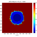
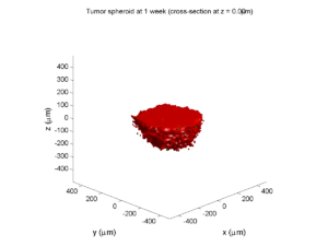
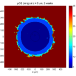
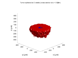
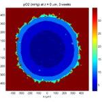
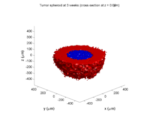
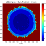
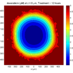
Here are some plots, showing (left from right) pO2 concentration, a cross-section of the tumor (red = live cells, green = apoptotic, and blue = necrotic), and the drug concentration (after start of therapy):
1 week:
Oxygen- and space-limited growth are restricted to the outer boundary of the tumor spheroid.
2 weeks:
Oxygenation is dipped below 5 mmHg in the center, leading to necrosis.
3 weeks:
As the tumor grows, the hypoxic gradient increases, and the necrotic core grows. The code turns on a constant 5 micromolar dose of doxorubicin at this point
Treatment + 12 hours:
The drug has started to penetrate the tumor, triggering apoptotic death towards the outer periphery where exposure has been greatest.
Treatment + 24 hours:
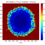
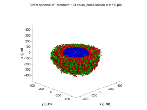
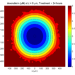
The drug profile hasn’t changed much, but the interior cells have now had greater exposure to drug, and hence greater response. Now apoptosis is observed throughout the non-necrotic tumor. The tumor has decreased in volume somewhat.
Treatment + 36 hours:
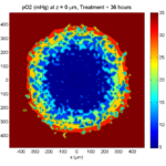
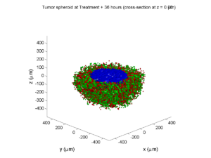
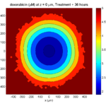
The non-necrotic tumor is now substantially apoptotic. We would require some pharamcokinetic effects (e.g., drug clearance, inactivation, or removal) to avoid the inevitable, presences of a pre-existing resistant strain, or emergence of resistance.
Treatment + 48 hours:
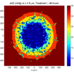
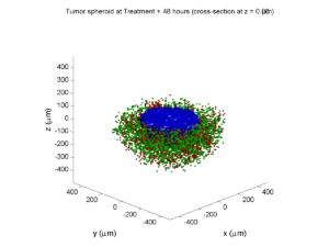

By now, almost all cells are apoptotic.
Treatment + 60 hours:
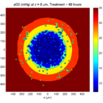
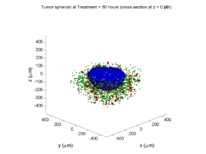
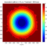
The non-necrotic tumor is nearly completed eliminated, leaving a leftover core of previously-necrotic cells (which did not change state in response to the drug–they were already dead!)
Source files
You can download completed source for this example here: https://sourceforge.net/projects/biofvm/files/Tutorials/Cellular_Automaton_1/
This file will include the following:
- BioFVM_cellular_automata.h
- BioFVM_cellular_automata.cpp
- BioFVM_CA_example_1.cpp
- read_MultiCellDS_xml.m (updated)
- plot_cellular_automata.m
- Makefile
What’s next
I plan to update this source code with extra cell motility, and potentially more realistic parameter values. Also, I plan to more formally separate out the example from the generic cell capabilities, so that this source code can work as a bona fide cellular automaton framework.
More immediately, my next tutorial will use the reverse strategy: start with an existing cellular automaton model, and integrate BioFVM capabilities.
Return to News • Return to MathCancer • Follow @MathCancer
Paul Macklin profiled in New Scientist article
Paul Macklin was recently featured in a New Scientist article on multidisciplinary jobs in cancer. It profiled the non-linear path he and others took to reach a multi-disciplinary career blending biology, mathematics, and computing.
Read the article: http://jobs.newscientist.com/article/knocking-cancer-out/ (Apr. 16, 2015)
Paul Macklin calls for common standards in cancer modeling
At a recent NCI-organized mini-symposium on big data in cancer, Paul Macklin called for new data standards in Multicellular data in simulations, experiments, and clinical science. USC featured the talk (abstract here) and the work at news.usc.edu.
Read the article: http://news.usc.edu/59091/usc-researcher-calls-for-common-standards-in-cancer-modeling/ (Feb. 21, 2014)
Paul Macklin interviewed at 2013 PSOC Annual Meeting
Paul Macklin gave a plenary talk at the 2013 NIH Physical Sciences in Oncology Annual Meeting. After the talk, he gave an interview to the Pauline Davies at the NIH on the need for data standards and model compatibility in computational and mathematical modeling of cancer. Of particular interest:
Pauline Davies: How would you ever get this standardization? Who would be responsible for saying we want it all reported in this particular way?
Paul Macklin: That’s a good question. It’s a bit of the chicken and the egg problem. Who’s going to come and give you data in your standard if you don’t have a standard? How do you plan a standard without any data? And so it’s a bit interesting. I just think someone needs to step forward and show leadership and try to get a small working group together, and at the end of the day, perfect is the enemy of the good. I think you start small and give it a go, and you add more to your standard as you need it. So maybe version one is, let’s say, how quickly the cells divide, how often they do it, how quickly they die, and what their oxygen level is, and maybe their positions. And that can be version one of this standard and a few of us try it out and see what we can do. I think it really comes down to a starting group of people and a simple starting point, and you grow it as you need it.
Shortly after, the MultiCellDS project was born (using just this strategy above!), with the generous assistance of the Breast Cancer Research Foundation.
Read / Listen to the interview: http://physics.cancer.gov/report/2013report/PaulMacklin.aspx (2013)
Macklin Lab featured on March 2013 cover of Notices of the American Mathematical Society
I’m very excited to be featured on this month’s cover of the Notices of the American Mathematical Society. The cover shows a series of images from a multiscale simulation of a tumor growing in the brain, made with John Lowengrub while I was a Ph.D. student at UC Irvine. (See Frieboes et al. 2007, Macklin et al. 2009, and Macklin and Lowengrub 2008.) The “about the cover” write-up (Page 325) gives more detail.
The inside has a short interview on our more current work, particularly 3-D agent-based modeling. You should also read Rick Durrett‘s perspective piece on cancer modeling (Page 304)—it’s a great read! (And yup, Figure 3 is from our patient-calibrated breast cancer modeling in Macklin et al. 2012. ;-) )
The entire March 2013 issue can be accessed for free at the AMS Notices website:
http://www.ams.org/notices/201303/
I want to thank Bill Casselman and Rick Durrett for making this possible. I had a lot of fun in the process, and I’m grateful for the opportunity to trade ideas!
DCIS modeling paper accepted
I am pleased to report that our paper has now been accepted. You can download the accepted preprint here. We also have a lot of supplementary material, including simulation movies, simulation datasets (for 0, 15, 30, adn 45 days of growth), and open source C++ code for postprocessing and visualization.
I discussed the results in detail here, but here’s the short version:
- We use a mechanistic, agent-based model of individual cancer cells growing in a duct. Cells are moved by adhesive and repulsive forces exchanged with other cells and the basement membrane. Cell phenotype is controlled by stochastic processes.
- We constrained all parameter expected to be relatively independent of patients by a careful analysis of the experimental biological and clinical literature.
- We developed the very first patient-specific calibration method, using clinically-accessible pathology. This is a key point in future patient-tailored predictions and surgical/therapeutic planning.
- The model made numerous quantitative predictions, such as:
- The tumor grows at a constant rate, between 7 to 10 mm/year. This is right in the middle of the range reported in the clinic.
- The tumor’s size in mammgraphy is linearly correlated with the post-surgical pathology size. When we linearly extrapolate our correlation across two orders of magnitude, it goes right through the middle of a cluster of 87 clinical data points.
- The tumor necrotic core has an age structuring: with oldest, calcified material in the center, and newest, most intact necrotic cells at the outer edge.
- The appearance of a “typical” DCIS duct cross-section varies with distance from the leading edge; all types of cross-sections predicted by our model are observed in patient pathology.
- The model also gave new insight on the underlying biology of breast cancer, such as:
- The split between the viable rim and necrotic core (observed almost universally in pathology) is not just an artifact, but an actual biomechanical effect from fast necrotic cell lysis.
- The constant rate of tumor growth arises from the biomechanical stress relief provided by lysing necrotic cells. This points to the critical role of intracellular and intra-tumoral water transport in determining the qualitative and quantitative behavior of tumors.
- Pyknosis (nuclear degradation in necrotic cells), must occur at a time scale between that of cell lysis (on the order of hours) and cell calcification (on the order of weeks).
- The current model cannot explain the full spectrum of calcification types; other biophysics, such as degradation over a long, 1-2 month time scale, must be at play.
Now hiring: Postdoctoral Researcher
I just posted a job opportunity for a postdoctoral researcher for computational modeling of breast, prostate, and metastatic cancer, with a heavy emphasis on calibrating (and validating!) to in vitro, in vivo, and clinical data.
If you’re a talented computational modeler and have a passion for applying mathematics to make a difference in clinical care, please read the job posting and apply!
(Note: Interested students in the Los Angeles/Orange County area may want to attend my applied math seminar talk at UCI next week to learn more about this work.)
