Category: agent-based model
Introducing cell interactions & transformations
Introduction
PhysiCell 1.10.0 introduces a number of new features designed to simplify modeling of complex interactions and transformations. This blog post will introduce the underlying mathematics and show a complete example. We will teach this and other examples in greater depth at our upcoming Virtual PhysiCell Workshop & Hackathon (July 24-30, 2022). (Apply here!!)
Cell Interactions
In the past, it has been possible to model complex cell-cell interactions (such as those needed for microecology and immunology) by connecting basic cell functions for interaction testing and custom functions. In particular, these functions were used for the COVID19 Coalition’s open source model of SARS-CoV-2 infections and immune responses. We now build upon that work to standardize and simplify these processes, making use of the cell’s state.neighbors (a list of all cells deemed to be within mechanical interaction distance).
All the parameters for cell-cell interactions are stored in cell.phenotype.cell_interactions.
Phagocytosis
A cell can phagocytose (ingest) another cell, with rates that vary with the cell’s live/dead status or the cell type. In particular, we store:
- double dead_phagocytosis_rate : This is the rate at which a cell can phagocytose a dead cell of any type.
std::vector<double> live_phagocytosis_rates: This is a vector of phagocytosis rates for live cells of specific types. If there are n cell definitions in the simulation, then there are n rates in this vector. Please note that the index i for any cell type is its index in the list of cell definitions, not necessarily the ID of its cell definition. For safety, use one of the following to determine that index:find_cell_definition_index( int type_ID ): search for the cell definition’s index by its type ID (cell.type)find_cell_definition_index( std::string type_name ): search for the cell definition’s index by its human-readable type name (cell.type_name)
We also supply a function to help access these live phagocytosis rates.
- double& live_phagocytosis_rate( std::string type_name ) : Directly access the cell’s rate of phagocytosing the live cell type by its human-readable name. For example,
pCell->phenotype.cell_interactions.live_phagocytosis_rate( "tumor cell" ) = 0.01;
At each mechanics time step (with duration \(\Delta t\), default 0.1 minutes), each cell runs through its list of neighbors. If the neighbor is dead, its probability of phagocytosing it between \(t\) and \(t+\Delta t\) is
\[ \verb+dead_phagocytosis_rate+ \cdot \Delta t\]
If the neighbor cell is alive and its type has index j, then its probability of phagocytosing the cell between \(t\) and \(t+\Delta t\) is
\[ \verb+live_phagocytosis_rates[j]+ \cdot \Delta t\]
PhysiCell’s standardized phagocytosis model does the following:
- The phagocytosing cell will absorb the phagocytosed cell’s total solid volume into the cytoplasmic solid volume
- The phagocytosing cell will absorb the phagocytosed cell’s total fluid volume into the fluid volume
- The phagocytosing cell will absorb all of the phagocytosed cell’s internalized substrates.
- The phagocytosed cell is set to zero volume, flagged for removal, and set to not mechanically interact with remaining cells.
- The phagocytosing cell does not change its target volume. The standard volume model will gradually “digest” the absorbed volume as the cell shrinks towards its target volume.
Cell Attack
A cell can attack (cause damage to) another live cell, with rates that vary with the cell’s type. In particular, we store:
- double damage_rate : This is the rate at which a cell causes (dimensionless) damage to a target cell. The cell’s total damage is stored in cell.state.damage. The total integrated attack time is stored in
cell.state.total_attack_time. std::vector<double> attack_rates: This is a vector of attack rates for live cells of specific types. If there are n cell definitions in the simulation, then there are n rates in this vector. Please note that the index i for any cell type is its index in the list of cell definitions, not necessarily the ID of its cell definition. For safety, use one of the following to determine that index:find_cell_definition_index( int type_ID ): search for the cell definition’s index by its type ID (cell.type)find_cell_definition_index( std::string type_name ): search for the cell definition’s index by its human-readable type name (cell.type_name)
We also supply a function to help access these attack rates.
- double& attack_rate( std::string type_name ) : Directly access the cell’s rate of attacking the live cell type by its human-readable name. For example,
pCell->phenotype.cell_interactions.attack_rate( "tumor cell" ) = 0.01;
At each mechanics time step (with duration \(\Delta t\), default 0.1 minutes), each cell runs through its list of neighbors. If the neighbor cell is alive and its type has index j, then its probability of attacking the cell between \(t\) and \(t+\Delta t\) is
\[ \verb+attack_rates[j]+ \cdot \Delta t\]
To attack the cell:
- The attacking cell will increase the target cell’s damage by \( \verb+damage_rate+ \cdot \Delta t\).
- The attacking cell will increase the target cell’s total attack time by \(\Delta t\).
Note that this allows us to have variable rates of damage (e.g., some immune cells may be “worn out”), and it allows us to distinguish between damage and integrated interaction time. (For example, you may want to write a model where damage can be repaired over time.)
As of this time, PhysiCell does not have a standardized model of death in response to damage. It is up to the modeler to vary a death rate with the total attack time or integrated damage, based on their hypotheses. For example:
\[ r_\textrm{apoptosis} = r_\textrm{apoptosis,0} + \left( r_\textrm{apoptosis,max} – r_\textrm{apoptosis,0} \right) \cdot \frac{ d^h }{ d_\textrm{halfmax}^h + d^h } \]
In a phenotype function, we might write this as:
void damage_response( Cell* pCell, Phenotype& phenotype, double dt )
{ // get the base apoptosis rate from our cell definition
     Cell_Definition* pCD = find_cell_definition( pCell->type_name );
     double apoptosis_0 = pCD->phenotype.death.rates[0];
     double apoptosis_max = 100 * apoptosis_0;
     double half_max = 2.0;
     double damage = pCell->state.damage;
     phenotype.death.rates[0] = apoptosis_0 +
(apoptosis_max -apoptosis_0) * Hill_response_function(d,half_max,1.0);
     return;
}
Cell Fusion
A cell can fuse with another live cell, with rates that vary with the cell’s type. In particular, we store:
std::vector<double> fusion_rates: This is a vector of fusion rates for live cells of specific types. If there are n cell definitions in the simulation, then there are n rates in this vector. Please note that the index i for any cell type is its index in the list of cell definitions, not necessarily the ID of its cell definition. For safety, use one of the following to determine that index:find_cell_definition_index( int type_ID ): search for the cell definition’s index by its type ID (cell.type)find_cell_definition_index( std::string type_name ): search for the cell definition’s index by its human-readable type name (cell.type_name)
We also supply a function to help access these fusion rates.
- double& fusion_rate( std::string type_name ) : Directly access the cell’s rate of fusing with the live cell type by its human-readable name. For example,
pCell->phenotype.cell_interactions.fusion_rate( "tumor cell" ) = 0.01;
At each mechanics time step (with duration \(\Delta t\), default 0.1 minutes), each cell runs through its list of neighbors. If the neighbor cell is alive and its type has index j, then its probability of fusing with the cell between \(t\) and \(t+\Delta t\) is
\[ \verb+fusion_rates[j]+ \cdot \Delta t\]
PhysiCell’s standardized fusion model does the following:
- The fusing cell will absorb the fused cell’s total cytoplasmic solid volume into the cytoplasmic solid volume
- The fusing cell will absorb the fused cell’s total nuclear volume into the nuclear solid volume
- The fusing cell will keep track of its number of nuclei in
state.number_of_nuclei. (So, if the fusing cell has 3 nuclei and the fused cell has 2 nuclei, then the new cell will have 5 nuclei.) - The fusing cell will absorb the fused cell’s total fluid volume into the fluid volume
- The fusing cell will absorb all of the fused cell’s internalized substrates.
- The fused cell is set to zero volume, flagged for removal, and set to not mechanically interact with remaining cells.
- The fused cell will be moved to the (volume weighted) center of mass of the two original cells.
- The fused cell does change its target volume to the sum of the original two cells’ target volumes. The combined cell will grow / shrink towards its new target volume.
Cell Transformations
A live cell can transform to another type (e.g., via differentiation). We store parameters for cell transformations in cell.phenotype.cell_transformations, particularly:
std::vector<double> transformation_rates: This is a vector of transformation rates from a cell’s current to type to one of the other cell types. If there are n cell definitions in the simulation, then there are n rates in this vector. Please note that the index i for any cell type is its index in the list of cell definitions, not necessarily the ID of its cell definition. For safety, use one of the following to determine that index:find_cell_definition_index( int type_ID ): search for the cell definition’s index by its type ID (cell.type)find_cell_definition_index( std::string type_name ): search for the cell definition’s index by its human-readable type name (cell.type_name)
We also supply a function to help access these transformation rates.
- double& transformation_rate( std::string type_name ) : Directly access the cell’s rate of transforming into a specific cell type by searching for its human-readable name. For example,
pCell->phenotype.cell_transformations.transformation_rate( "mutant tumor cell" ) = 0.01;
At each phenotype time step (with duration \(\Delta t\), default 6 minutes), each cell runs through the vector of transformation rates. If a (different) cell type has index j, then the cell’s probability transforming to that type between \(t\) and \(t+\Delta t\) is
\[ \verb+transformation_rates[j]+ \cdot \Delta t\]
PhysiCell uses the built-in Cell::convert_to_cell_definition( Cell_Definition& ) for the transformation.
Other New Features
This release also includes a number of handy new features:
Advanced Chemotaxis
After setting chemotaxis sensitivities in phenotype.motility and enabling the feature, cells can chemotax based on linear combinations of substrate gradients.
std::vector<double> phenotype.motility.chemotactic_sensitivitiesis a vector of chemotactic sensitivities, one for each substrate in the environment. By default, these are all zero for backwards compatibility. A positive sensitivity denotes chemotaxis up a corresponding substrate’s gradient (towards higher values), whereas a negative sensitivity gives chemotaxis against a gradient (towards lower values).- For convenience, you can access (read and write) a substrate’s chemotactic sensitivity via
phenotype.motility.chemotactic_sensitivity(name)wherenameis the human-readable name of a substrate in the simulation. - If the user sets
cell.cell_functions.update_migration_bias = advanced_chemotaxis_function, then these sensitivities are used to set the migration bias direction via: \[\vec{d}_\textrm{mot} = s_0 \nabla \rho_0 + \cdots + s_n \nabla \rho_n. \] - If the user sets
cell.cell_functions.update_migration_bias = advanced_chemotaxis_function_normalized, then these sensitivities are used to set the migration bias direction via: \[\vec{d}_\textrm{mot} = s_0 \frac{\nabla\rho_0}{|\nabla\rho_0|} + \cdots + s_n \frac{ \nabla \rho_n }{|\nabla\rho_n|}.\]
Cell Adhesion Affinities
cell.phenotype.mechanics.adhesion_affinitiesis a vector of adhesive affinities, one for each cell type in the simulation. By default, these are all one for backwards compatibility.- For convenience, you can access (read and write) a cell’s adhesive affinity for a specific cell type via
phenotype.mechanics.adhesive_affinity(name), wherenameis the human-readable name of a cell type in the simulation. - The standard mechanics function (based on potentials) uses this as follows. If cell
ihas an cell-cell adhesion strengtha_iand an adhesive affinityp_ijto cell typej, and if celljhas a cell-cell adhesion strength ofa_jand an adhesive affinityp_jito cell typei, then the strength of their adhesion is \[ \sqrt{ a_i p_{ij} \cdot a_j p_{ji} }.\] Notice that if \(a_i = a_j\) and \(p_{ij} = p_{ji}\), then this reduces to \(a_i a_{pj}\). - The standard elastic spring function (
standard_elastic_contact_function) uses this as follows. If cellihas an elastic constanta_iand an adhesive affinityp_ijto cell typej, and if celljhas an elastic constanta_jand an adhesive affinityp_jito cell typei, then the strength of their adhesion is \[ \sqrt{ a_i p_{ij} \cdot a_j p_{ji} }.\] Notice that if \(a_i = a_j\) and \(p_{ij} = p_{ji}\), then this reduces to \(a_i a_{pj}\).
Signal and Behavior Dictionaries
We will talk about this in the next blog post. See http://www.mathcancer.org/blog/introducing-cell-signal-and-behavior-dictionaries.
A brief immunology example
We will illustrate the major new functions with a simplified cancer-immune model, where tumor cells attract macrophages, which in turn attract effector T cells to damage and kill tumor cells. A mutation process will transform WT cancer cells into mutant cells that can better evade this immune response.
The problem:
We will build a simplified cancer-immune system to illustrate the new behaviors.
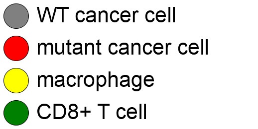
- WT cancer cells: Proliferate and release a signal that will stimulate an immune response. Cancer cells can transform into mutant cancer cells. Dead cells release debris. Damage increases apoptotic cell death.
- Mutant cancer cells: Proliferate but release less of the signal, as a model of immune evasion. Dead cells release debris. Damage increases apoptotic cell death.
- Macrophages: Chemotax towards the tumor signal and debris, and release a pro-inflammatory signal. They phagocytose dead cells.
- CD8+ T cells: Chemotax towards the pro-inflammatory signal and cause damage to tumor cells. As a model of immune evasion, CD8+ T cells can damage WT cancer cells faster than mutant cancer cells.
We will use the following diffusing factors:
- Tumor signal: Released by WT and mutant cells at different rates. We’ll fix a 1 min\(^{-1}\) decay rate and set the diffusion parameter to 10000 \(\mu m^2/\)min to give a 100 micron diffusion length scale.
- Pro-inflammatory signal: Released by macrophages. We’ll fix a 1 min\(^{-1}\) decay rate and set the diffusion parameter to 10000 \(\mu;m^2/\)min to give a 100 micron diffusion length scale.
- Debris: Released by dead cells. We’ll fix a 0.01 min\(^{-1}\) decay rate and choose a diffusion coefficient of 1 \(\mu;m^2/\)min for a 10 micron diffusion length scale.
In particular, we won’t worry about oxygen or resources in this model. We can use Neumann (no flux) boundary conditions.
Getting started with a template project and the graphical model builder
The PhysiCell Model Builder was developed by Randy Heiland and undergraduate researchers at Indiana University to help ease the creation of PhysiCell models, with a focus on generating correct XML configuration files that define the diffusing substrates and cell definitions. Here, we assume that you have cloned (or downloaded) the repository adjacent to your PhysiCell repository. (So that the path to PMB from PhysiCell’s root directory is ../PhysiCell-model-builder/).
Let’s start a new project (starting with the template project) from a command prompt or shell in the PhysiCell directory, and then open the model builder.
make template
make
python ../PhysiCell-model-builder/bin/pmb.py
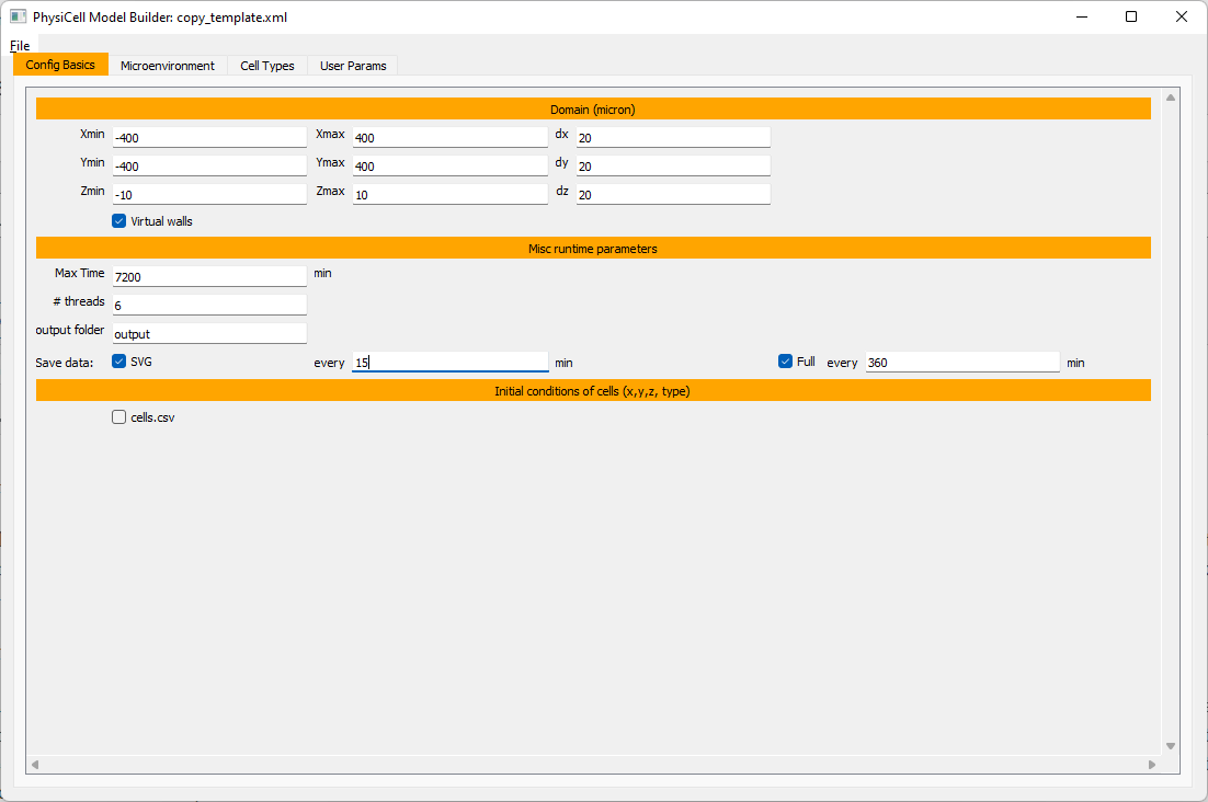
Setting up the domain
Let’s use a [-400,400] x [-400,400] 2D domain, with “virtual walls” enabled (so cells stay in the domain). We’ll run for 5760 minutes (4 days), saving SVG outputs every 15 minutes.
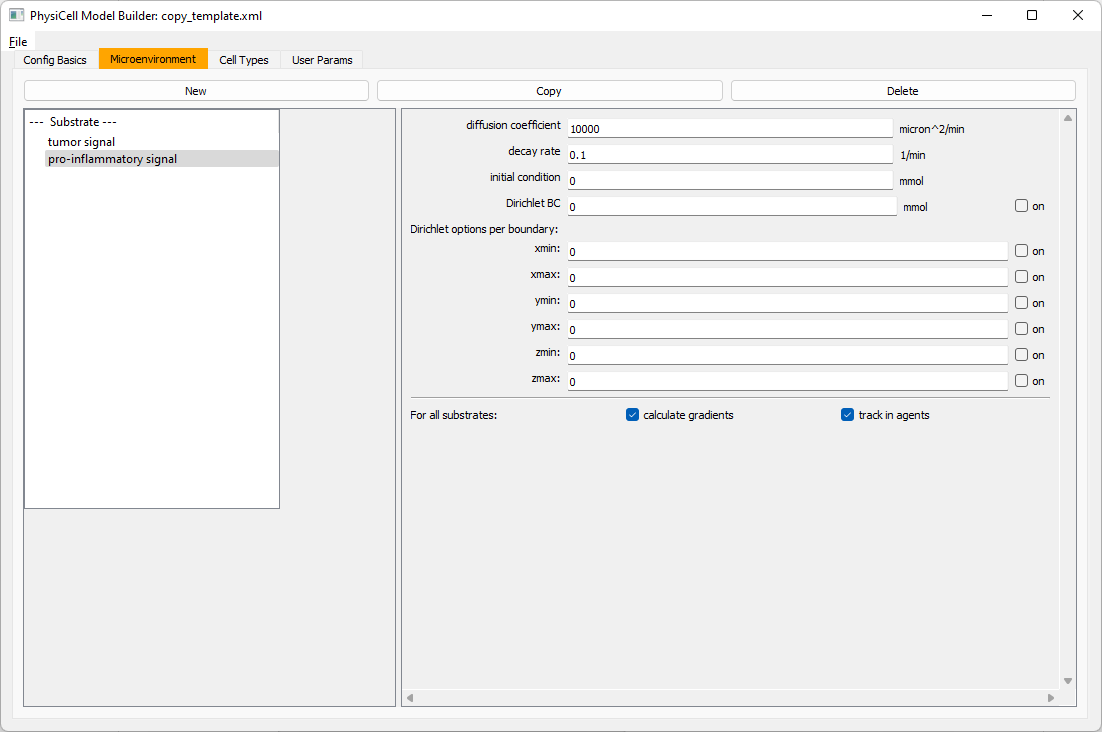
Setting up diffusing substrates
Move to the microenvironment tab. Click on substrate and rename it to tumor signal . Set the decay rate to 0.1 and diffusion parameter to 10000. Uncheck the Dirichlet condition box so that it’s a zero-flux (Neumann) boundary condition.
 Now, select
 tumor signal in the lefthand column, click copy, and rename the new substrate (substrate01) to pro-inflammatory signal with the same parameters.
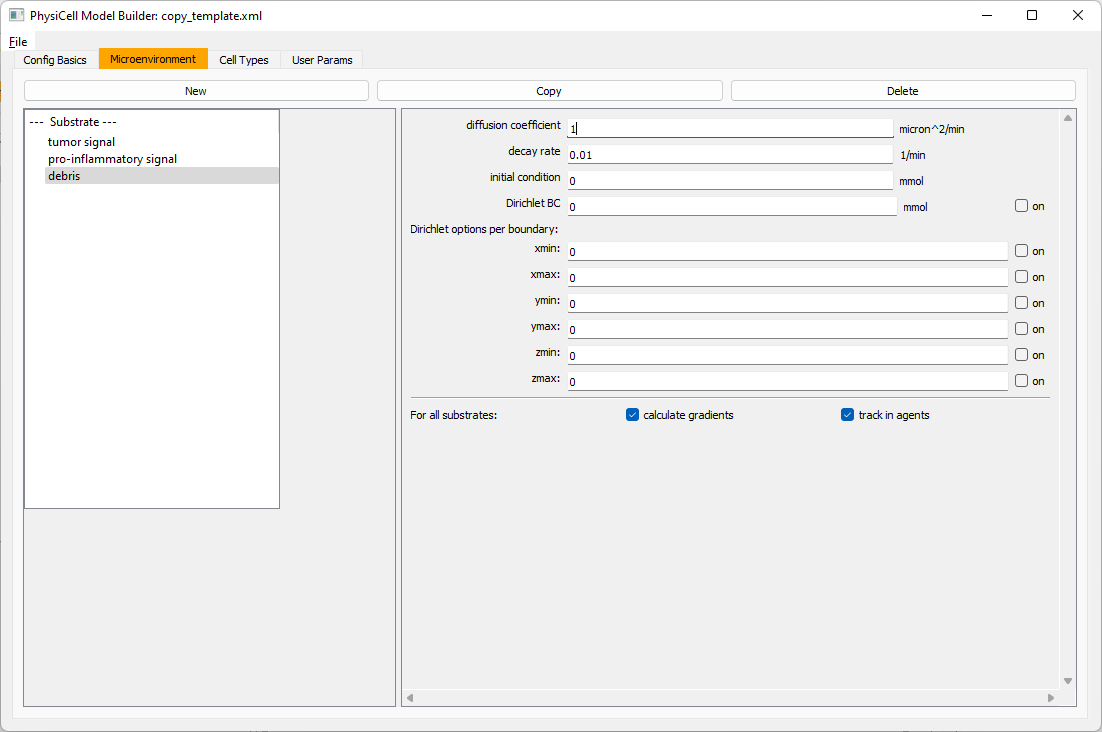
Then, copy this substrate one more time, and rename it from name debris. Set its decay rate to 0.01, and its diffusion parameter to 1.
Let’s save our work before continuing. Go to File, Save as, and save it as PhysiCell_settings.xml in your config file. (Go ahead and overwrite.)
If model builder crashes, you can reopen it, then go to File, Open, and select this file to continue editing.
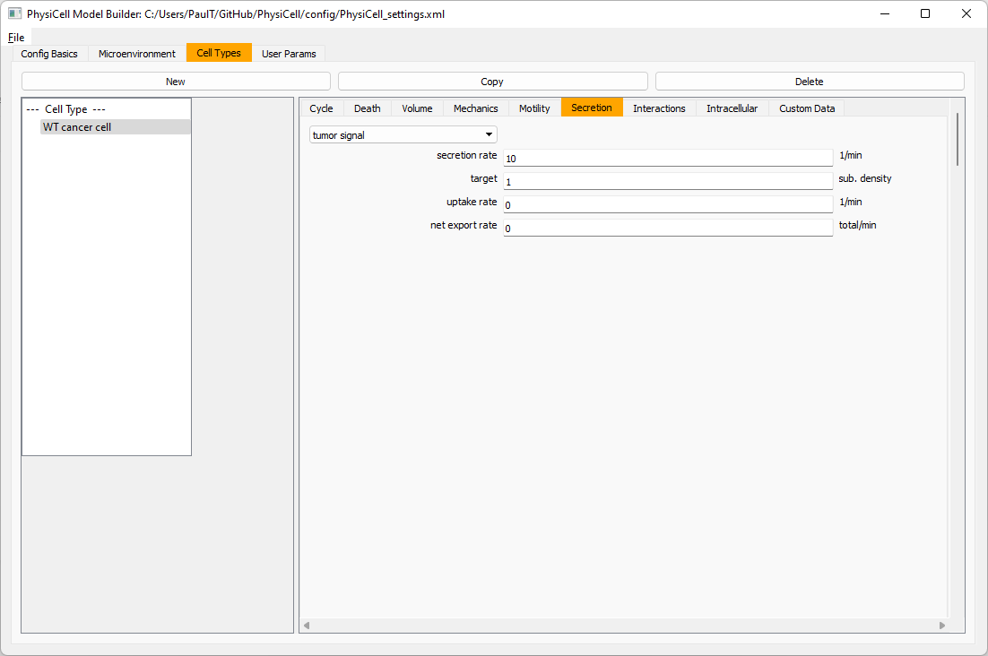
Setting up the WT cancer cells
Move to the cell types tab. Click on the default cell type on the left side, and rename it to WT cancer cell. Leave most of the parameter values at their defaults. Move to the secretion sub-tab (in phenotype). From the drop-down menu, select tumor signal. Let’s set a high secretion rate of 10.
We’ll need to set WT cells as able to mutate, but before that, the model builder needs to “know” about that cell type. So, let’s move on to the next cell type for now.
Setting up mutant tumor cells
Click the WT cancer cell in the left column, and click copy. Rename this cell type (for me, it’s cell_def03) to mutant cancer cell. Click the secretion sub-tab, and set its secretion rate of tumor signal lower to 0.1.
Set the WT mutation rate
Now that both cell types are in the simulation, we can set up mutation. Let’s suppose the mean time to a mutation is 10000 minutes, or a rate of 0.0001 min\(^{-1}\).
Click the WT cancer cell in the left column to select it. Go to the interactions tab. Go down to transformation rate, and choose mutant cancer cell from the drop-down menu. Set its rate to 0.0001.

Create macrophages
Now click on the WT cancer cell type in the left column, and click copy to create a new cell type. Click on the new type (for me cell_def04) and rename it to macrophage.
Click on cycle and change to a live cells and change from a duration representation to a transition rate representation. Keep its cycling rate at 0.
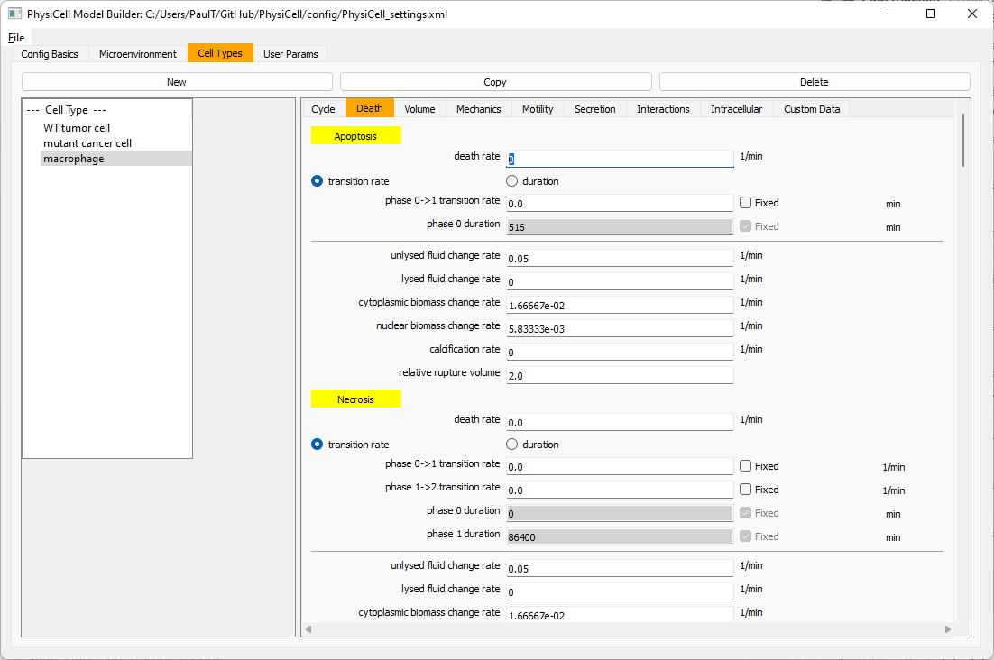
Go to death and change from duration to transition rate for both apoptosis and necrosis, and keep the death rates at 0.0
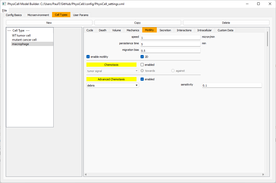
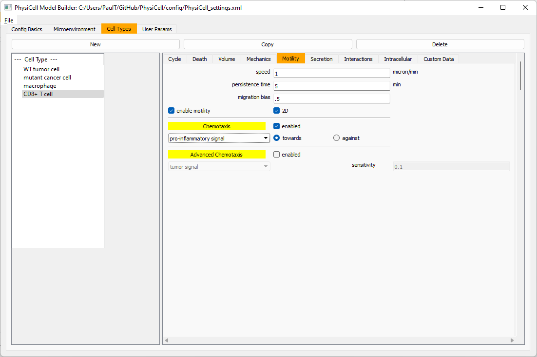
Now, go to the motility tab. Set the speed to 1 \(\mu m/\)min, persistence time to 5 min, and migration bias to 0.5. Be sure to enable motility. Then, enable advanced motility. Choose tumor signal from the drop-down and set its sensitivity to 1.0. Then choose debris from the drop-down and set its sensitivity to 0.1
Now, let’s make sure it secretes pro-inflammatory signal. Go to the secretion tab. Choose tumor signal from the drop-down, and make sure its secretion rate is 0. Then choose pro-inflammatory signal from the drop-down, set its secretion rate to 100, and its target value to 1.

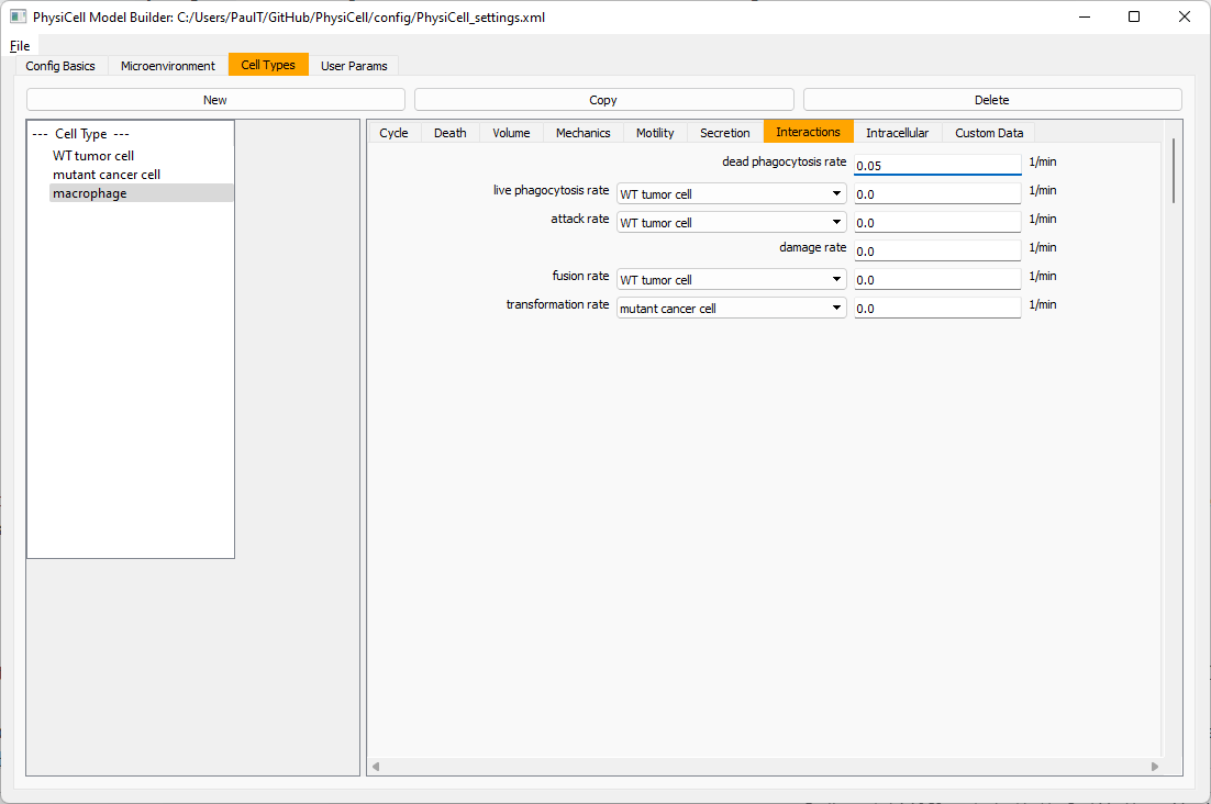
Lastly, let’s set macrophages up to phagocytose dead cells. Go to the interactions tab. Set the dead phagocytosis rate to 0.05 (so that the mean contact time to wait to eat a dead cell is 1/0.05 = 20 minutes). This would be a good time to save your work.
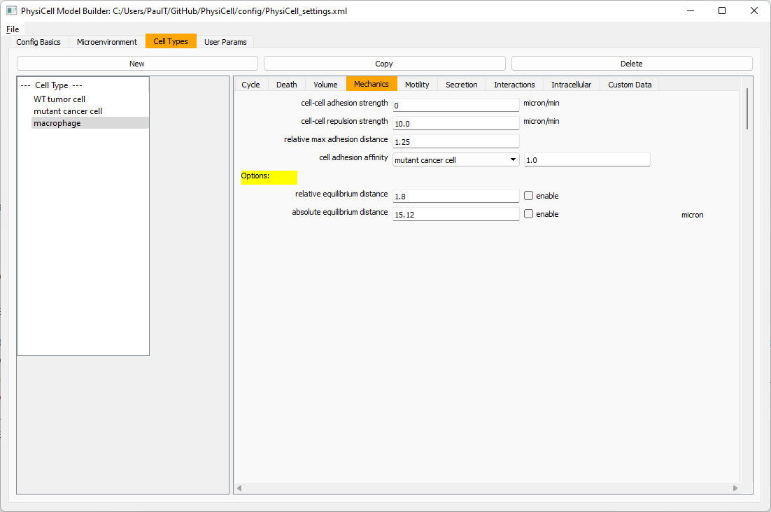
Macrophages probably shouldn’t be adhesive. So go to the mechanics sub-tab, and set the cell-cell adhesion strength to 0.0.
Create CD8+ T cells
Select macrophage on the left column, and choose copy. Rename the new cell type to CD8+ T cell. Go to the secretion sub-tab and make sure to set the secretion rate of pro-inflammatory signal to 0.0.
Now, let’s use simpler chemotaxis for these towards pro-inflammatory signal. Go to the motility tab. Uncheck advanced chemotaxis and check chemotaxis. Choose pro-inflammatory signal from the drop-down, with the towards option.
Lastly, let’s set these cells to attack WT and tumor cells. Go to the interactions tab. Set the dead phagocytosis rate to 0.
Now, let’s work on attack. Set the damage rate to 1.0. Near attack rate, choose WT tumor cell from the drop-down, and set its attack rate to 10 (so it attacks during any 0.1 minute interval). Then choose mutant tumor cell from the drop-down, and set its attack rate to 1 (as a model of immune evasion, where they are less likely to attack a non-WT tumor cell).

Set the initial cell conditions
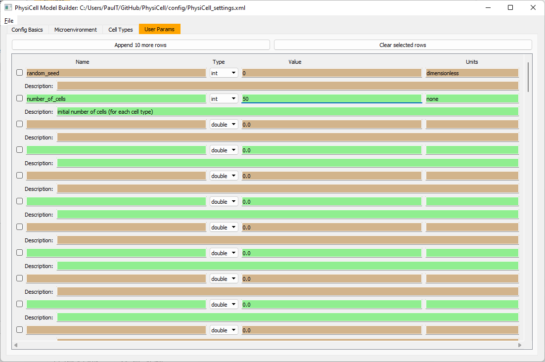
Go to the user params tab. On number of cells, choose 50. It will randomly place 50 of each cell type at the start of the simulation.
That’s all! Go to File and save (or save as), and overwrite config/PhysiCell_settings.xml. Then close the model builder.
Testing the model
Go into the PhysiCell directory. Since you already compiled, just run your model (which will use PhysiCell_settings.xml that you just saved to the config directory). For Linux or MacOS (or similar Unix-like systems):
./project
Windows users would type project without the ./ at the front.
Take a look at your SVG outputs in the output directory. You might consider making an animated gif (make gif) or a movie:
make jpeg && make movie
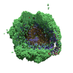
Here’s what we have.
 |
Promising! But we still need to write a little C++ so that damage kills tumor cells, and so that dead tumor cells release debris. (And we could stand to “anchor” tumor cells to ECM so they don’t get pushed around by the immune cells, but that’s a post for another day!)
Customizing the WT and mutant tumor cells with phenotype functions
First, open custom.h in the custom_modules directory, and declare a function for tumor phenotype:
void tumor_phenotype_function( Cell* pCell, Phenotype& phenotype, double dt );
Now, let’s open custom.cpp to write this function at the bottom. Here’s what we’ll do:
- If dead, set rate of debris release to 1.0 and return.
- Otherwise, we’ll set damage-based apoptosis.
- Get the base apoptosis rate
- Get the current damage
- Use a Hill response function with a half-max of 36, max apoptosis rate of 0.05 min\(^{-1}\), and a hill power of 2.0
Here’s the code:
void tumor_phenotype_function( Cell* pCell, Phenotype& phenotype, double dt )
{
   // find my cell definition
   static Cell_Definition* pCD = find_cell_definition( pCell->type_name );

   // find the index of debris in the environment
   static int nDebris = microenvironment.find_density_index( "debris" );
   static int nTS = microenvironment.find_density_index( "tumor signal" );

   // if dead: release debris. stop releasing tumor signal
   if( phenotype.death.dead == true )
   {
      phenotype.secretion.secretion_rates[nDebris] = 1;
      phenotype.secretion.saturation_densities[nDebris] = 1;

      phenotype.secretion.secretion_rates[nTS] = 0;

      // last time I'll execute this function (special optional trick)
      pCell->functions.update_phenotype = NULL;
      return;
   }

   // damage increases death

   // find death model
   static int nApoptosis =
      phenotype.death.find_death_model_index( PhysiCell_constants::apoptosis_death_model );

   double signal = pCell->state.damage; // current damage
   double base_val = pCD->phenotype.death.rates[nApoptosis]; // base death rate (from cell def)
   double max_val = 0.05; // max death rate (at large damage)

   static double damage_halfmax = 36.0;
   double hill_power = 2.0;

   // evaluate Hill response function
   double hill = Hill_response_function( signal , damage_halfmax , hill_power );
   // set "dose-dependent" death rate
   phenotype.death.rates[nApoptosis] = base_val + (max_val-base_val)*hill;

   return;
}
Now, we need to make sure we apply these functions to tumor cell. Go to `create_cell_types` and look just before we display the cell definitions. We need to:
- Search for the WT tumor cell definition
- Set the update_phenotype function for that type to the tumor_phenotype_function we just wrote
- Repeat for the mutant tumor cell type.
Here’s the code:
...
   /*
      Put any modifications to individual cell definitions here.

      This is a good place to set custom functions.
   */

   cell_defaults.functions.update_phenotype = phenotype_function;
   cell_defaults.functions.custom_cell_rule = custom_function;
   cell_defaults.functions.contact_function = contact_function;

   Cell_Definition* pCD = find_cell_definition( "WT cancer cell");
   pCD->functions.update_phenotype = tumor_phenotype_function;

   pCD = find_cell_definition( "mutant cancer cell");
   pCD->functions.update_phenotype = tumor_phenotype_function;

   /*
      This builds the map of cell definitions and summarizes the setup.
   */

   display_cell_definitions( std::cout );
   return;
}
That’s it! Let’s recompile and run!
make && ./project
And here’s the final movie.
|
Much better! Now the
Coming up next!
We will use the signal and behavior dictionaries to help us easily write C++ functions to modulate the tumor and immune cell behaviors.
Once ready, this will be posted at http://www.mathcancer.org/blog/introducing-cell-signal-and-behavior-dictionaries/.
PhysiCell Tools : PhysiCell-povwriter
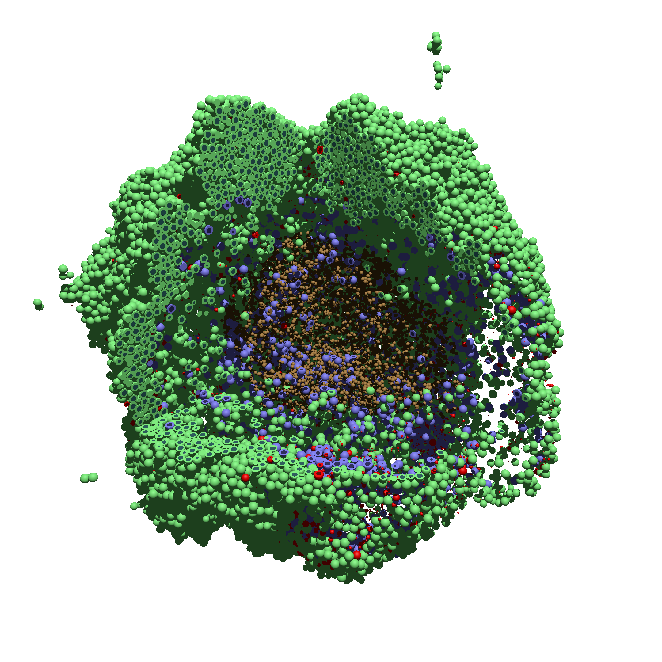
As PhysiCell matures, we are starting to turn our attention to better training materials and an ecosystem of open source PhysiCell tools. PhysiCell-povwriter is is designed to help transform your 3-D simulation results into 3-D visualizations like this one:
PhysiCell-povwriter transforms simulation snapshots into 3-D scenes that can be rendered into still images using POV-ray: an open source software package that uses raytracing to mimic the path of light from a source of illumination to a single viewpoint (a camera or an eye). The result is a beautifully rendered scene (at any resolution you choose) with very nice shading and lighting.
If you repeat this on many simulation snapshots, you can create an animation of your work.
What you’ll need
This workflow is entirely based on open source software:
- 3-D simulation data (likely stored in ./output from your project)
- PhysiCell-povwriter, available on GitHub at
- POV-ray, available at
- ImageMagick (optional, for image file conversions)
- mencoder (optional, for making compressed movies)
Setup
Building PhysiCell-povwriter
After you clone PhysiCell-povwriter or download its source from a release, you’ll need to compile it. In the project’s root directory, compile the project by:
make
(If you need to set up a C++ PhysiCell development environment, click here for OSX or here for Windows.)
Next, copy povwriter (povwriter.exe in Windows) to either the root directory of your PhysiCell project, or somewhere in your path. Copy ./config/povwriter-settings.xml to the ./config directory of your PhysiCell project.
Editing resolutions in POV-ray
PhysiCell-povwriter is intended for creating “square” images, but POV-ray does not have any pre-created square rendering resolutions out-of-the-box. However, this is straightforward to fix.
- Open POV-Ray
- Go to the “tools” menu and select “edit resolution INI file”
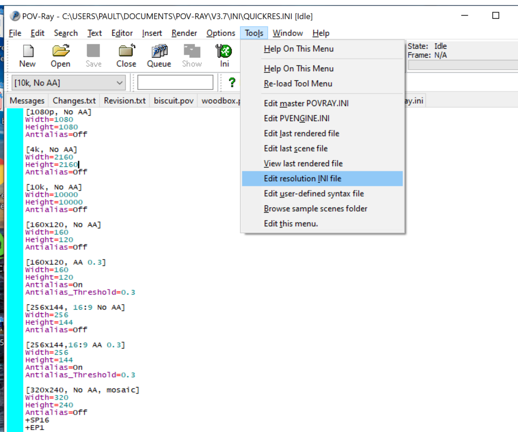
- At the top of the INI file (which opens for editing in POV-ray), make a new profile:
[1080x1080, AA]
Width=480
Height=480
Antialias=On
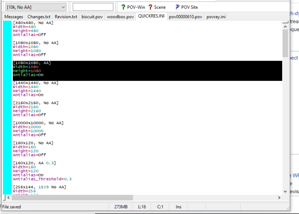
- Make similar profiles (with unique names) to suit your preferences. I suggest one at 480×480 (as a fast preview), another at 2160×2160, and another at 5000×5000 (because they will be absurdly high resolution). For example:
[2160x2160 no AA]
Width=2160
Height=2160
Antialias=Off
You can optionally make more profiles with antialiasing on (which provides some smoothing for areas of high detail), but you’re probably better off just rendering without antialiasing at higher resolutions and the scaling the image down as needed. Also, rendering without antialiasing will be faster.
- Once done making profiles, save and exit POV-Ray.
- The next time you open POV-Ray, your new resolution profiles will be available in the lefthand dropdown box.


Configuring PhysiCell-povwriter
Once you have copied povwriter-settings.xml to your project’s config file, open it in a text editor. Below, we’ll show the different settings.
Camera settings
<camera>
	<distance_from_origin units="micron">1500</distance_from_origin>
	<xy_angle>3.92699081699</xy_angle> <!-- 5*pi/4 -->
	<yz_angle>1.0471975512</yz_angle> <!-- pi/3 -->
</camera>
For simplicity, PhysiCell-POVray (currently) always aims the camera towards the origin (0,0,0), with “up” towards the positive z-axis. distance_from_origin sets how far the camera is placed from the origin. xy_angle sets the angle \(\theta\) from the positive x-axis in the xy-plane. yz_angle sets the angle \(\phi\) from the positive z-axis in the yz-plane. Both angles are in radians.
Options
<options>
	<use_standard_colors>true</use_standard_colors>
	<nuclear_offset units="micron">0.1</nuclear_offset>
	<cell_bound units="micron">750</cell_bound>
	<threads>8</threads>
</options>
use_standard_colors (if set to true) uses a built-in “paint-by-numbers” color scheme, where each cell type (identified with an integer) gets XML-defined colors for live, apoptotic, and dead cells. More on this below. If use_standard_colors is set to false, then PhysiCell-povwriter uses the my_pigment_and_finish_function in ./custom_modules/povwriter.cpp to color cells.
The nuclear_offset is a small additional height given to nuclei when cropping to avoid visual artifacts when rendering (which can cause some “tearing” or “bleeding” between the rendered nucleus and cytoplasm). cell_bound is used for leaving some cells out of bound: any cell with |x|, |y|, or |z| exceeding cell_bound will not be rendered. threads is used for parallelizing on multicore processors; note that it only speeds up povwriter if you are converting multiple PhysiCell outputs to povray files.
Save
<save> <!-- done -->
	<folder>output</folder> <!-- use . for root -->
	<filebase>output</filebase>
	<time_index>3696</time_index>
</save>
Use folder to tell PhysiCell-povwriter where the data files are stored. Use filebase to tell how the outputs are named. Typically, they have the form output########_cells_physicell.mat; in this case, the filebase is output. Lastly, use time_index to set the output number. For example if your file is output00000182_cells_physicell.mat, then filebase = output and time_index = 182.
Below, we’ll see how to specify ranges of indices at the command line, which would supersede the time_index given here in the XML.
Clipping planes
PhysiCell-povwriter uses clipping planes to help create cutaway views of the simulations. By default, 3 clipping planes are used to cut out an octant of the viewing area.
Recall that a plane can be defined by its normal vector n and a point p on the plane. With these, the plane can be defined as all points x satisfying
\[ \left( \vec{x} -\vec{p} \right) \cdot \vec{n} = 0 \]
These are then written out as a plane equation
\[ a x + by + cz + d = 0, \]
where
\[ (a,b,c) = \vec{n} \hspace{.5in} \textrm{ and } \hspace{0.5in} d = \: – \vec{n} \cdot \vec{p}. \]
As of Version 1.0.0, we are having some difficulties with clipping planes that do not pass through the origin (0,0,0), for which \( d = 0 \).
In the config file, these planes are written as \( (a,b,c,d) \):
<clipping_planes> <!-- done -->
	<clipping_plane>0,-1,0,0</clipping_plane>
	<clipping_plane>-1,0,0,0</clipping_plane>
	<clipping_plane>0,0,1,0</clipping_plane>
</clipping_planes>
Note that cells “behind” the plane (where \( ( \vec{x} – \vec{p} ) \cdot \vec{n} \le 0 \)) are rendered, and cells in “front” of the plane (where \( (\vec{x}-\vec{p}) \cdot \vec{n} > 0 \)) are not rendered. Cells that intersect the plane are partially rendered (using constructive geometry via union and intersection commands in POV-ray).
Cell color definitions
Within <cell_color_definitions>, you’ll find multiple <cell_colors> blocks, each of which defines the live, dead, and necrotic colors for a specific cell type (with the type ID indicated in the attribute). These colors are only applied if use_standard_colors is set to true in options. See above.
The live colors are given as two rgb (red,green,blue) colors for the cytoplasm and nucleus of live cells. Each element of this triple can range from 0 to 1, and not from 0 to 255 as in many raw image formats. Next, finish specifies ambient (how much highly-scattered background ambient light illuminates the cell), diffuse (how well light rays can illuminate the surface), and specular (how much of a shiny reflective splotch the cell gets).
See the POV-ray documentation for for information on the finish.
This is repeated to give the apoptotic and necrotic colors for the cell type.
<cell_colors type="0">
	<live>
		<cytoplasm>.25,1,.25</cytoplasm> <!-- red,green,blue -->
		<nuclear>0.03,0.125</nuclear>
		<finish>0.05,1,0.1</finish> <!-- ambient,diffuse,specular -->
	</live>
	<apoptotic>
		<cytoplasm>1,0,0</cytoplasm> <!-- red,green,blue -->
		<nuclear>0.125,0,0</nuclear>
		<finish>0.05,1,0.1</finish> <!-- ambient,diffuse,specular -->
	</apoptotic>
	<necrotic>
		<cytoplasm>1,0.5412,0.1490</cytoplasm> <!-- red,green,blue -->
		<nuclear>0.125,0.06765,0.018625</nuclear>
		<finish>0.01,0.5,0.1</finish> <!-- ambient,diffuse,specular -->
	</necrotic>
</cell_colors>
Use multiple cell_colors blocks (each with type corresponding to the integer cell type) to define the colors of multiple cell types.
Using PhysiCell-povwriter
Use by the XML configuration file alone
The simplest syntax:
physicell$ ./povwriter
(Windows users: povwriter or povwriter.exe) will process ./config/povwriter-settings.xml and convert the single indicated PhysiCell snapshot to a .pov file.
If you run POV-writer with the default configuration file in the povwriter structure (with the supplied sample data), it will render time index 3696 from the immunotherapy example in our 2018 PhysiCell Method Paper:
physicell$ ./povwriter

povwriter version 1.0.0
================================================================================

Copyright (c) Paul Macklin 2019, on behalf of the PhysiCell project
OSI License: BSD-3-Clause (see LICENSE.txt)

Usage:
================================================================================
povwriter : run povwriter with config file ./config/settings.xml

povwriter FILENAME.xml : run povwriter with config file FILENAME.xml

povwriter x:y:z : run povwriter on data in FOLDER with indices from x
to y in incremenets of z

Example: ./povwriter 0:2:10 processes files:
./FOLDER/FILEBASE00000000_physicell_cells.mat
./FOLDER/FILEBASE00000002_physicell_cells.mat
...
./FOLDER/FILEBASE00000010_physicell_cells.mat
(See the config file to set FOLDER and FILEBASE)

povwriter x1,...,xn : run povwriter on data in FOLDER with indices x1,...,xn

Example: ./povwriter 1,3,17 processes files:
./FOLDER/FILEBASE00000001_physicell_cells.mat
./FOLDER/FILEBASE00000003_physicell_cells.mat
./FOLDER/FILEBASE00000017_physicell_cells.mat
(Note that there are no spaces.)
(See the config file to set FOLDER and FILEBASE)

Code updates at https://github.com/PhysiCell-Tools/PhysiCell-povwriter

Tutorial & documentation at http://MathCancer.org/blog/povwriter
================================================================================

Using config file ./config/povwriter-settings.xml ...
Using standard coloring function ...
Found 3 clipping planes ...
Found 2 cell color definitions ...
Processing file ./output/output00003696_cells_physicell.mat...
Matrix size: 32 x 66978
Creating file pov00003696.pov for output ...
Writing 66978 cells ...
done!

Done processing all 1 files!
The result is a single POV-ray file (pov00003696.pov) in the root directory.
Now, open that file in POV-ray (double-click the file if you are in Windows), choose one of your resolutions in your lefthand dropdown (I’ll choose 2160×2160 no antialiasing), and click the green “run” button.
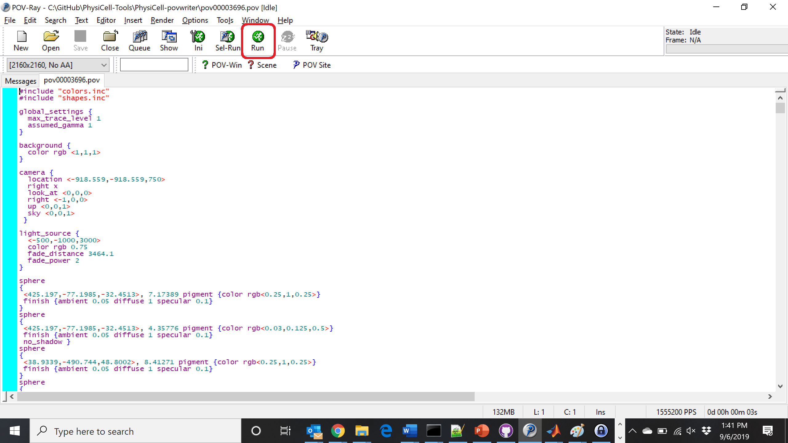
You can watch the image as it renders. The result should be a PNG file (named pov00003696.png) that looks like this:
Using command-line options to process multiple times (option #1)
Now, suppose we have more outputs to process. We still state most of the options in the XML file as above, but now we also supply a command-line argument in the form of start:interval:end. If you’re still in the povwriter project, note that we have some more sample data there. Let’s grab and process it:
physicell$ cd output
physicell$ unzip more_samples.zip
Archive: more_samples.zip
inflating: output00000000_cells_physicell.mat
inflating: output00000001_cells_physicell.mat
inflating: output00000250_cells_physicell.mat
inflating: output00000300_cells_physicell.mat
inflating: output00000500_cells_physicell.mat
inflating: output00000750_cells_physicell.mat
inflating: output00001000_cells_physicell.mat
inflating: output00001250_cells_physicell.mat
inflating: output00001500_cells_physicell.mat
inflating: output00001750_cells_physicell.mat
inflating: output00002000_cells_physicell.mat
inflating: output00002250_cells_physicell.mat
inflating: output00002500_cells_physicell.mat
inflating: output00002750_cells_physicell.mat
inflating: output00003000_cells_physicell.mat
inflating: output00003250_cells_physicell.mat
inflating: output00003500_cells_physicell.mat
inflating: output00003696_cells_physicell.mat

physicell$ ls

citation and license.txt
more_samples.zip
output00000000_cells_physicell.mat
output00000001_cells_physicell.mat
output00000250_cells_physicell.mat
output00000300_cells_physicell.mat
output00000500_cells_physicell.mat
output00000750_cells_physicell.mat
output00001000_cells_physicell.mat
output00001250_cells_physicell.mat
output00001500_cells_physicell.mat
output00001750_cells_physicell.mat
output00002000_cells_physicell.mat
output00002250_cells_physicell.mat
output00002500_cells_physicell.mat
output00002750_cells_physicell.mat
output00003000_cells_physicell.mat
output00003250_cells_physicell.mat
output00003500_cells_physicell.mat
output00003696.xml
output00003696_cells_physicell.mat
Let’s go back to the parent directory and run povwriter:
physicell$ ./povwriter 0:250:3500

povwriter version 1.0.0
================================================================================

Copyright (c) Paul Macklin 2019, on behalf of the PhysiCell project
OSI License: BSD-3-Clause (see LICENSE.txt)

Usage:
================================================================================
povwriter : run povwriter with config file ./config/settings.xml

povwriter FILENAME.xml : run povwriter with config file FILENAME.xml

povwriter x:y:z : run povwriter on data in FOLDER with indices from x
to y in incremenets of z

Example: ./povwriter 0:2:10 processes files:
./FOLDER/FILEBASE00000000_physicell_cells.mat
./FOLDER/FILEBASE00000002_physicell_cells.mat
...
./FOLDER/FILEBASE00000010_physicell_cells.mat
(See the config file to set FOLDER and FILEBASE)

povwriter x1,...,xn : run povwriter on data in FOLDER with indices x1,...,xn

Example: ./povwriter 1,3,17 processes files:
./FOLDER/FILEBASE00000001_physicell_cells.mat
./FOLDER/FILEBASE00000003_physicell_cells.mat
./FOLDER/FILEBASE00000017_physicell_cells.mat
(Note that there are no spaces.)
(See the config file to set FOLDER and FILEBASE)

Code updates at https://github.com/PhysiCell-Tools/PhysiCell-povwriter

Tutorial & documentation at http://MathCancer.org/blog/povwriter
================================================================================

Using config file ./config/povwriter-settings.xml ...
Using standard coloring function ...
Found 3 clipping planes ...
Found 2 cell color definitions ...
Matrix size: 32 x 18317
Processing file ./output/output00000000_cells_physicell.mat...
Creating file pov00000000.pov for output ...
Writing 18317 cells ...
Processing file ./output/output00002000_cells_physicell.mat...
Matrix size: 32 x 33551
Creating file pov00002000.pov for output ...
Writing 33551 cells ...
Processing file ./output/output00002500_cells_physicell.mat...
Matrix size: 32 x 43440
Creating file pov00002500.pov for output ...
Writing 43440 cells ...
Processing file ./output/output00001500_cells_physicell.mat...
Matrix size: 32 x 40267
Creating file pov00001500.pov for output ...
Writing 40267 cells ...
Processing file ./output/output00003000_cells_physicell.mat...
Matrix size: 32 x 56659
Creating file pov00003000.pov for output ...
Writing 56659 cells ...
Processing file ./output/output00001000_cells_physicell.mat...
Matrix size: 32 x 74057
Creating file pov00001000.pov for output ...
Writing 74057 cells ...
Processing file ./output/output00003500_cells_physicell.mat...
Matrix size: 32 x 66791
Creating file pov00003500.pov for output ...
Writing 66791 cells ...
Processing file ./output/output00000500_cells_physicell.mat...
Matrix size: 32 x 114316
Creating file pov00000500.pov for output ...
Writing 114316 cells ...
done!

Processing file ./output/output00000250_cells_physicell.mat...
Matrix size: 32 x 75352
Creating file pov00000250.pov for output ...
Writing 75352 cells ...
done!

Processing file ./output/output00002250_cells_physicell.mat...
Matrix size: 32 x 37959
Creating file pov00002250.pov for output ...
Writing 37959 cells ...
done!

Processing file ./output/output00001750_cells_physicell.mat...
Matrix size: 32 x 32358
Creating file pov00001750.pov for output ...
Writing 32358 cells ...
done!

Processing file ./output/output00002750_cells_physicell.mat...
Matrix size: 32 x 49658
Creating file pov00002750.pov for output ...
Writing 49658 cells ...
done!

Processing file ./output/output00003250_cells_physicell.mat...
Matrix size: 32 x 63546
Creating file pov00003250.pov for output ...
Writing 63546 cells ...
done!

done!

done!

done!

Processing file ./output/output00001250_cells_physicell.mat...
Matrix size: 32 x 54771
Creating file pov00001250.pov for output ...
Writing 54771 cells ...
done!

done!

done!

done!

Processing file ./output/output00000750_cells_physicell.mat...
Matrix size: 32 x 97642
Creating file pov00000750.pov for output ...
Writing 97642 cells ...
done!

done!

Done processing all 15 files!
Notice that the output appears a bit out of order. This is normal: povwriter is using 8 threads to process 8 files at the same time, and sending some output to the single screen. Since this is all happening simultaneously, it’s a bit jumbled (and non-sequential). Don’t panic. You should now have created pov00000000.pov, pov00000250.pov, … , pov00003500.pov.
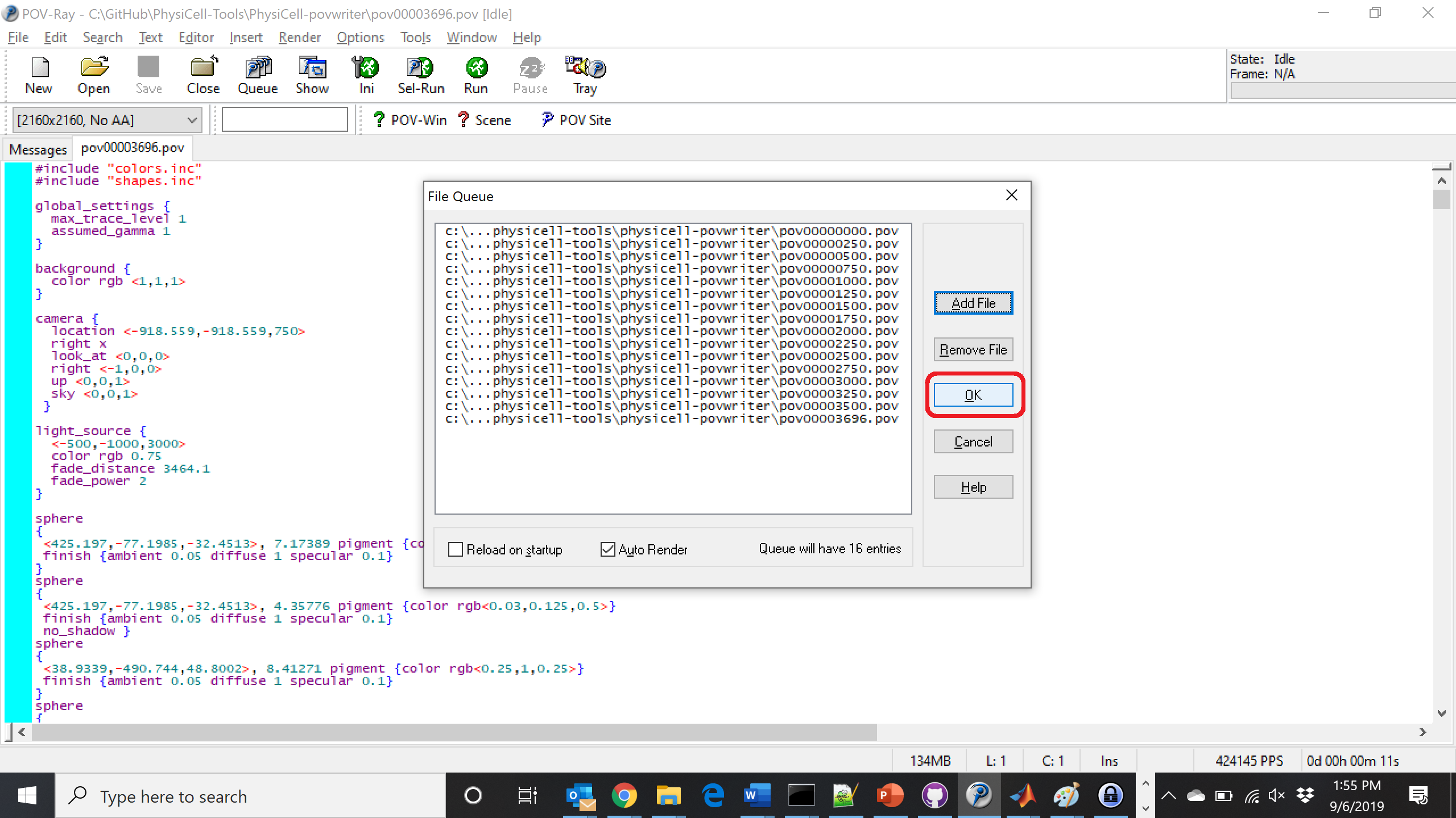
Now, go into POV-ray, and choose “queue.” Click “Add File” and select all 15 .pov files you just created:
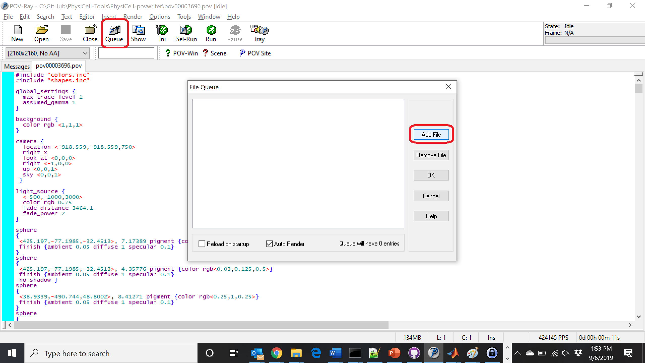
Hit “OK” to let it render all the povray files to create PNG files (pov00000000.png, … , pov00003500.png).
Using command-line options to process multiple times (option #2)
You can also give a list of indices. Here’s how we render time indices 250, 1000, and 2250:
physicell$ ./povwriter 250,1000,2250

povwriter version 1.0.0
================================================================================

Copyright (c) Paul Macklin 2019, on behalf of the PhysiCell project
OSI License: BSD-3-Clause (see LICENSE.txt)

Usage:
================================================================================
povwriter : run povwriter with config file ./config/settings.xml

povwriter FILENAME.xml : run povwriter with config file FILENAME.xml

povwriter x:y:z : run povwriter on data in FOLDER with indices from x
to y in incremenets of z

Example: ./povwriter 0:2:10 processes files:
./FOLDER/FILEBASE00000000_physicell_cells.mat
./FOLDER/FILEBASE00000002_physicell_cells.mat
...
./FOLDER/FILEBASE00000010_physicell_cells.mat
(See the config file to set FOLDER and FILEBASE)

povwriter x1,...,xn : run povwriter on data in FOLDER with indices x1,...,xn

Example: ./povwriter 1,3,17 processes files:
./FOLDER/FILEBASE00000001_physicell_cells.mat
./FOLDER/FILEBASE00000003_physicell_cells.mat
./FOLDER/FILEBASE00000017_physicell_cells.mat
(Note that there are no spaces.)
(See the config file to set FOLDER and FILEBASE)

Code updates at https://github.com/PhysiCell-Tools/PhysiCell-povwriter

Tutorial & documentation at http://MathCancer.org/blog/povwriter
================================================================================

Using config file ./config/povwriter-settings.xml ...
Using standard coloring function ...
Found 3 clipping planes ...
Found 2 cell color definitions ...
Processing file ./output/output00002250_cells_physicell.mat...
Matrix size: 32 x 37959
Creating file pov00002250.pov for output ...
Writing 37959 cells ...
Processing file ./output/output00001000_cells_physicell.mat...
Matrix size: 32 x 74057
Creating file pov00001000.pov for output ...
Processing file ./output/output00000250_cells_physicell.mat...
Matrix size: 32 x 75352
Writing 74057 cells ...
Creating file pov00000250.pov for output ...
Writing 75352 cells ...
done!

done!

done!

Done processing all 3 files!
This will create files pov00000250.pov, pov00001000.pov, and pov00002250.pov. Render them in POV-ray just as before.
Advanced options (at the source code level)
If you set use_standard_colors to false, povwriter uses the function my_pigment_and_finish_function (at the end of ./custom_modules/povwriter.cpp). Make sure that you set colors.cyto_pigment (RGB) and colors.nuclear_pigment (also RGB). The source file in povwriter has some hinting on how to write this. Note that the XML files saved by PhysiCell have a legend section that helps you do determine what is stored in each column of the matlab file.
Optional postprocessing
Image conversion / manipulation with ImageMagick
Suppose you want to convert the PNG files to JPEGs, and scale them down to 60% of original size. That’s very straightforward in ImageMagick:
physicell$ magick mogrify -format jpg -resize 60% pov*.png
Creating an animated GIF with ImageMagick
Suppose you want to create an animated GIF based on your images. I suggest first converting to JPG (see above) and then using ImageMagick again. Here, I’m adding a 20 ms delay between frames:
physicell$ magick convert -delay 20 *.jpg out.gif
Here’s the result:
Creating a compressed movie with Mencoder
Syntax coming later.
Closing thoughts and future work
In the future, we will probably allow more control over the clipping planes and a bit more debugging on how to handle planes that don’t pass through the origin. (First thoughts: we need to change how we use union and intersection commands in the POV-ray outputs.)
We should also look at adding some transparency for the cells. I’d prefer something like rgba (red-green-blue-alpha), but POV-ray uses filters and transmission, and we want to make sure to get it right.
Lastly, it would be nice to find a balance between the current very simple camera setup and better control.
Thanks for reading this PhysiCell Friday tutorial! Please do give PhysiCell at try (at http://PhysiCell.org) and read the method paper at PLoS Computational Biology.
Working with PhysiCell MultiCellDS digital snapshots in Matlab

PhysiCell 1.2.1 and later saves data as a specialized MultiCellDS digital snapshot, which includes chemical substrate fields, mesh information, and a readout of the cells and their phenotypes at single simulation time point. This tutorial will help you learn to use the matlab processing files included with PhysiCell.
This tutorial assumes you know (1) how to work at the shell / command line of your operating system, and (2) basic plotting and other functions in Matlab.
Key elements of a PhysiCell digital snapshot
A PhysiCell digital snapshot (a customized form of the MultiCellDS digital simulation snapshot) includes the following elements saved as XML and MAT files:
- output12345678.xml : This is the “base” output file, in MultiCellDS format. It includes key metadata such as when the file was created, the software, microenvironment information, and custom data saved at the simulation time. The Matlab files read this base file to find other related files (listed next). Example: output00003696.xml
- initial_mesh0.mat : This is the computational mesh information for BioFVM at time 0.0. Because BioFVM and PhysiCell do not use moving meshes, we do not save this data at any subsequent time.
- output12345678_microenvironment0.mat : This saves each biochemical substrate in the microenvironment at the computational voxels defined in the mesh (see above). Example: output00003696_microenvironment0.mat
- output12345678_cells.mat : This saves very basic cellular information related to BioFVM, including cell positions, volumes, secretion rates, uptake rates, and secretion saturation densities. Example: output00003696_cells.mat
- output12345678_cells_physicell.mat : This saves extra PhysiCell data for each cell agent, including volume information, cell cycle status, motility information, cell death information, basic mechanics, and any user-defined custom data. Example: output00003696_cells_physicell.mat
These snapshots make extensive use of Matlab Level 4 .mat files, for fast, compact, and well-supported saving of array data. Note that even if you cannot ready MultiCellDS XML files, you can work to parse the .mat files themselves.
The PhysiCell Matlab .m files
Every PhysiCell distribution includes some matlab functions to work with PhysiCell digital simulation snapshots, stored in the matlab subdirectory. The main ones are:
- composite_cutaway_plot.m : provides a quick, coarse 3-D cutaway plot of the discrete cells, with different colors for live (red), apoptotic (b), and necrotic (black) cells.
- read_MultiCellDS_xml.m : reads the “base” PhysiCell snapshot and its associated matlab files.
- set_MCDS_constants.m : creates a data structure MCDS_constants that has the same constants as PhysiCell_constants.h. This is useful for identifying cell cycle phases, etc.
- simple_cutaway_plot.m : provides a quick, coarse 3-D cutaway plot of user-specified cells.
- simple_plot.m : provides, a quick, coarse 3-D plot of the user-specified cells, without a cutaway or cross-sectional clipping plane.
A note on GNU Octave
Unfortunately, GNU octave does not include XML file parsing without some significant user tinkering. And one you’re done, it is approximately one order of magnitude slower than Matlab. Octave users can directly import the .mat files described above, but without the helpful metadata in the XML file. We’ll provide more information on the structure of these MAT files in a future blog post. Moreover, we plan to provide python and other tools for users without access to Matlab.
A sample digital snapshot
We provide a 3-D simulation snapshot from the final simulation time of the cancer-immune example in Ghaffarizadeh et al. (2017, in review) at:
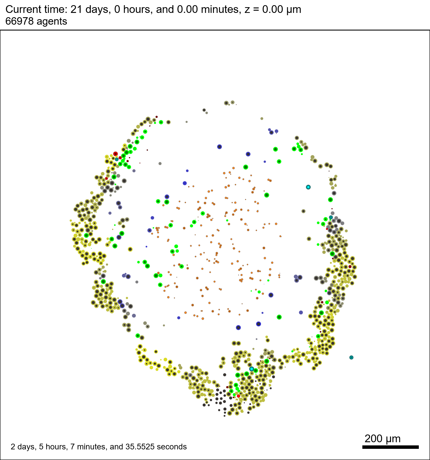
The corresponding SVG cross-section for that time (through z = 0 μm) looks like this:
Unzip the sample dataset in any directory, and make sure the matlab files above are in the same directory (or in your Matlab path). If you’re inside matlab:
!unzip 3D_PhysiCell_matlab_sample.zip
Loading a PhysiCell MultiCellDS digital snapshot
Now, load the snapshot:
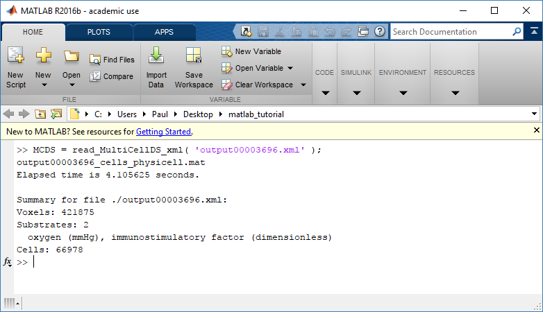
MCDS = read_MultiCellDS_xml( 'output00003696.xml');
This will load the mesh, substrates, and discrete cells into the MCDS data structure, and give a basic summary:
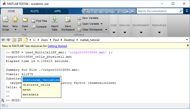
Typing ‘MCDS’ and then hitting ‘tab’ (for auto-completion) shows the overall structure of MCDS, stored as metadata, mesh, continuum variables, and discrete cells:
To get simulation metadata, such as the current simulation time, look at MCDS.metadata.current_time
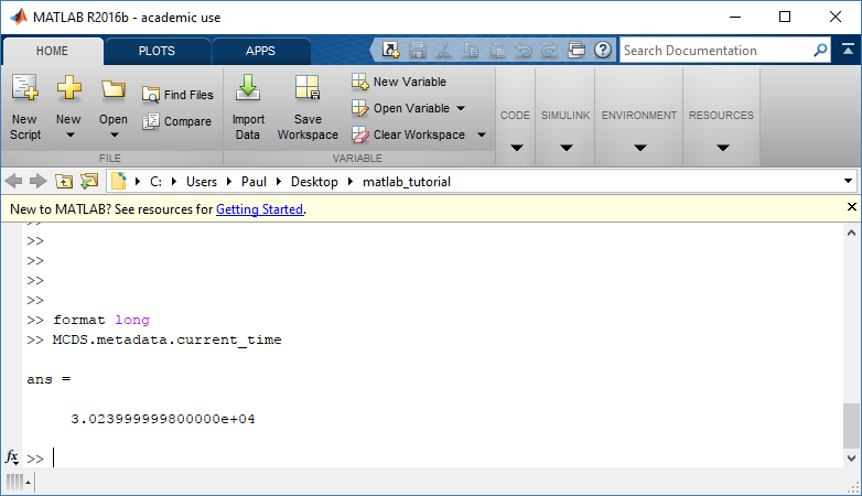
Here, we see that the current simulation time is 30240 minutes, or 21 days. MCDS.metadata.current_runtime gives the elapsed walltime to up to this point: about 53 hours (1.9e5 seconds), including file I/O time to write full simulation data once per 3 simulated minutes after the start of the adaptive immune response.
Plotting chemical substrates
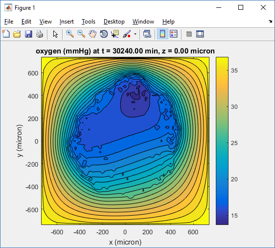
Let’s make an oxygen contour plot through z = 0 μm. First, we find the index corresponding to this z-value:
k = find( MCDS.mesh.Z_coordinates == 0 );
Next, let’s figure out which variable is oxygen. Type “MCDS.continuum_variables.name”, which will show the array of variable names:
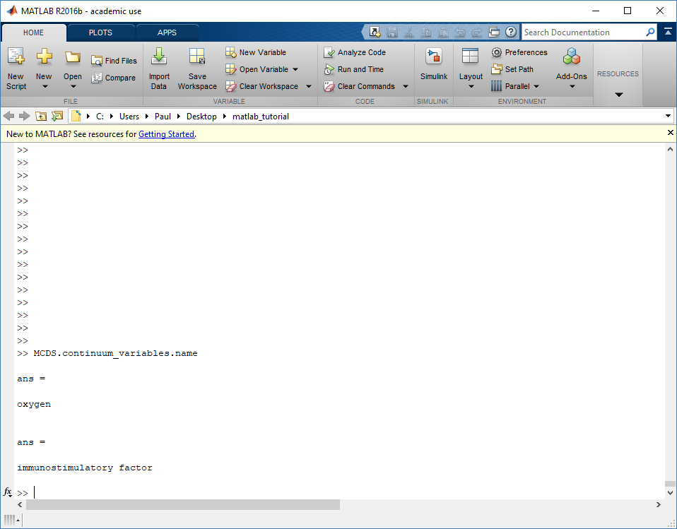
Here, oxygen is the first variable, (index 1). So, to make a filled contour plot:
contourf( MCDS.mesh.X(:,:,k), MCDS.mesh.Y(:,:,k), ...
     MCDS.continuum_variables(1).data(:,:,k) , 20 ) ;
Now, let’s set this to a correct aspect ratio (no stretching in x or y), add a colorbar, and set the axis labels, using
metadata to get labels:
axis image
colorbar
xlabel( sprintf( 'x (%s)' , MCDS.metadata.spatial_units) );
ylabel( sprintf( 'y (%s)' , MCDS.metadata.spatial_units) );
Lastly, let’s add an appropriate (time-based) title:
title( sprintf('%s (%s) at t = %3.2f %s, z = %3.2f %s', MCDS.continuum_variables(1).name , ...
     MCDS.continuum_variables(1).units , ...
     MCDS.metadata.current_time , ...
     MCDS.metadata.time_units, ...
     MCDS.mesh.Z_coordinates(k), ...
     MCDS.metadata.spatial_units ) );
Here’s the end result:
We can easily export graphics, such as to PNG format:
print( '-dpng' , 'output_o2.png' );
For more on plotting BioFVM data, see the tutorial
at http://www.mathcancer.org/blog/saving-multicellds-data-from-biofvm/
Plotting cells in space
3-D point cloud
First, let’s plot all the cells in 3D:
plot3( MCDS.discrete_cells.state.position(:,1) , MCDS.discrete_cells.state.position(:,2), ...
	MCDS.discrete_cells.state.position(:,3) , 'bo' );
At first glance, this does not look good: some cells are far out of the simulation domain, distorting the automatic range of the plot:
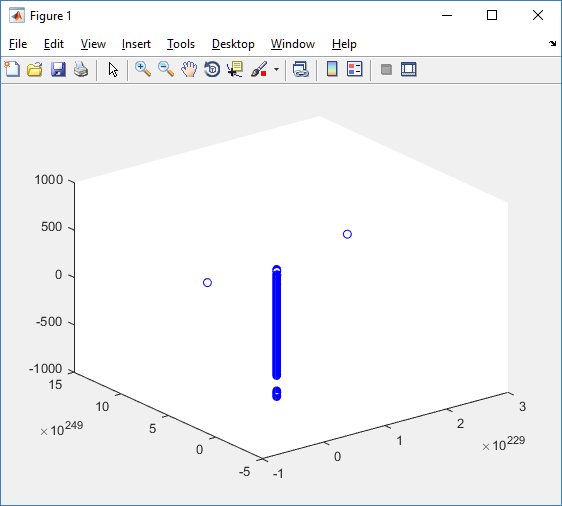
This does not ordinarily happen in PhysiCell (the default cell mechanics functions have checks to prevent such behavior), but this example includes a simple Hookean elastic adhesion model for immune cell attachment to tumor cells. In rare circumstances, an attached tumor cell or immune cell can apoptose on its own (due to its background apoptosis rate),
without “knowing” to detach itself from the surviving cell in the pair. The remaining cell attempts to calculate its elastic velocity based upon an invalid cell position (no longer in memory), creating an artificially large velocity that “flings” it out of the simulation domain. Such cells are not simulated any further, so this is effectively equivalent to an extra apoptosis event (only 3 cells are out of the simulation domain after tens of millions of cell-cell elastic adhesion calculations). Future versions of this example will include extra checks to prevent this rare behavior.
The plot can simply be fixed by changing the axis:
axis( 1000*[-1 1 -1 1 -1 1] )
axis square
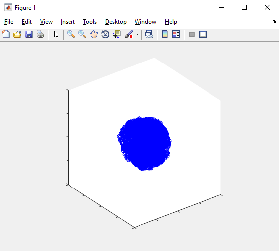
Notice that this is a very difficult plot to read, and very non-interactive (laggy) to rotation and scaling operations. We can make a slightly nicer plot by searching for different cell types and plotting them with different colors:
% make it easier to work with the cell positions;
P = MCDS.discrete_cells.state.position;

% find type 1 cells
ind1 = find( MCDS.discrete_cells.metadata.type == 1 );
% better still, eliminate those out of the simulation domain
ind1 = find( MCDS.discrete_cells.metadata.type == 1 & ...
    abs(P(:,1))' < 1000 & abs(P(:,2))' < 1000 & abs(P(:,3))' < 1000 );

% find type 0 cells
ind0 = find( MCDS.discrete_cells.metadata.type == 0 & ...
    abs(P(:,1))' < 1000 & abs(P(:,2))' < 1000 & abs(P(:,3))' < 1000 );

%now plot them
P = MCDS.discrete_cells.state.position;
plot3( P(ind0,1), P(ind0,2), P(ind0,3), 'bo' )
hold on
plot3( P(ind1,1), P(ind1,2), P(ind1,3), 'ro' )
hold off
axis( 1000*[-1 1 -1 1 -1 1] )
axis square
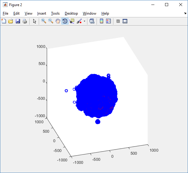
However, this isn’t much better. You can use the scatter3 function to gain more control on the size and color of the plotted cells, or even make macros to plot spheres in the cell locations (with shading and lighting), but Matlab is very slow when plotting beyond 103 cells. Instead, we recommend the faster preview functions below for data exploration, and higher-quality plotting (e.g., by POV-ray) for final publication-
Fast 3-D cell data previewers
Notice that plot3 and scatter3 are painfully slow for any nontrivial number of cells. We can use a few fast previewers to quickly get a sense of the data. First, let’s plot all the dead cells, and make them red:
clf
simple_plot( MCDS,  MCDS, MCDS.discrete_cells.dead_cells , 'r' )
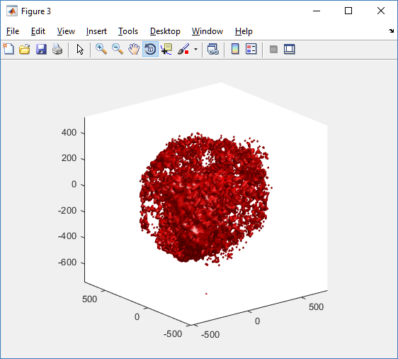
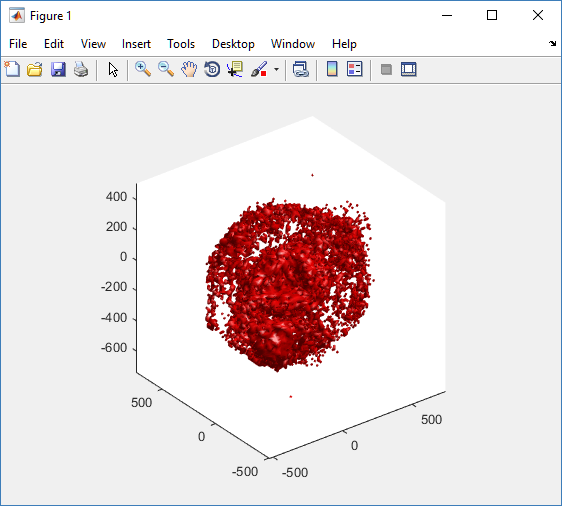
This function creates a coarse-grained 3-D indicator function (0 if no cells are present; 1 if they are), and plots a 3-D level surface. It is very responsive to rotations and other operations to explore the data. You may notice the second argument is a list of indices: only these cells are plotted. This gives you a method to select cells with specific characteristics when plotting. (More on that below.) If you want to get a sense of the interior structure, use a cutaway plot:
clf
simple_cutaway_plot( MCDS, MCDS, MCDS.discrete_cells.dead_cells , 'r' )
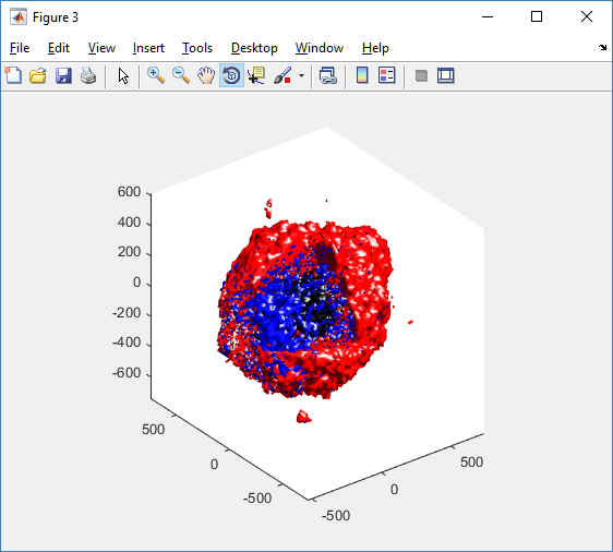
We also provide a fast “composite” cutaway which plots all live cells as red, apoptotic cells as blue (without the cutaway), and all necrotic cells as black:
clf
composite_cutaway_plot( MCDS )
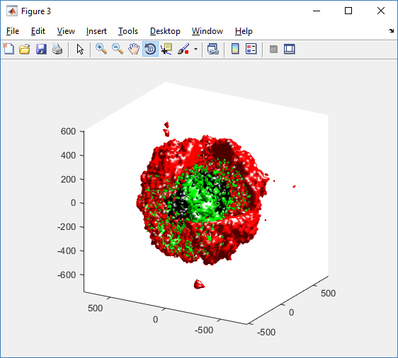
Lastly, we show an improved plot that uses different colors for the immune cells, and Matlab’s “find” function to help set up the indexing:
constants = set_MCDS_constants

% find the type 0 necrotic cells
ind0_necrotic = find( MCDS.discrete_cells.metadata.type == 0 & ...
    (MCDS.discrete_cells.phenotype.cycle.current_phase == constants.necrotic_swelling | ...
    MCDS.discrete_cells.phenotype.cycle.current_phase == constants.necrotic_lysed | ...
    MCDS.discrete_cells.phenotype.cycle.current_phase == constants.necrotic) );

% find the live type 0 cells
ind0_live = find( MCDS.discrete_cells.metadata.type == 0 & ...
    (MCDS.discrete_cells.phenotype.cycle.current_phase ~= constants.necrotic_swelling & ...
    MCDS.discrete_cells.phenotype.cycle.current_phase ~= constants.necrotic_lysed & ...
    MCDS.discrete_cells.phenotype.cycle.current_phase ~= constants.necrotic & ...
    MCDS.discrete_cells.phenotype.cycle.current_phase ~= constants.apoptotic) );

clf
% plot live tumor cells red, in cutaway view
simple_cutaway_plot( MCDS, ind0_live , 'r' );
hold on
% plot dead tumor cells black, in cutaway view
simple_cutaway_plot( MCDS, ind0_necrotic , 'k' )
% plot all immune cells, but without cutaway (to show how they infiltrate)
simple_plot( MCDS, ind1, 'g' )
hold off
A small cautionary note on future compatibility
PhysiCell 1.2.1 uses the <custom> data tag (allowed as part of the MultiCellDS specification) to encode its cell data, to allow a more compact data representation, because the current PhysiCell daft does not support such a formulation, and Matlab is painfully slow at parsing XML files larger than ~50 MB. Thus, PhysiCell snapshots are not yet fully compatible with general MultiCellDS tools, which would by default ignore custom data. In the future, we will make available converter utilities to transform “native” custom PhysiCell snapshots to MultiCellDS snapshots that encode all the cellular information in a more verbose but compatible XML format.
Closing words and future work
Because Octave is not a great option for parsing XML files (with critical MultiCellDS metadata), we plan to write similar functions to read and plot PhysiCell snapshots in Python, as an open source alternative. Moreover, our lab in the next year will focus on creating further MultiCellDS configuration, analysis, and visualization routines. We also plan to provide additional 3-D functions for plotting the discrete cells and varying color with their properties.
In the longer term, we will develop open source, stand-alone analysis and visualization tools for MultiCellDS snapshots (including PhysiCell snapshots). Please stay tuned!
Running the PhysiCell sample projects
Introduction
In PhysiCell 1.2.1 and later, we include four sample projects on cancer heterogeneity, bioengineered multicellular systems, and cancer immunology. This post will walk you through the steps to build and run the examples.
If you are new to PhysiCell, you should first make sure you’re ready to run it. (Please note that this applies in particular for OSX users, as Xcode’s g++ is not compatible out-of-the-box.) Here are tutorials on getting ready to Run PhysiCell:
- Setting up a 64-bit gcc environment in Windows.
- Setting up gcc / OpenMP on OSX (MacPorts edition)
- Setting up gcc / OpenMP on OSX (Homebrew edition)
Note: This is the preferred method for Mac OSX. - Getting started with a PhysiCell Virtual Appliance (for virtual machines like VirtualBox)
Note: The “native” setups above are preferred, but the Virtual Appliance is a great “plan B” if you run into trouble
Please note that we expect to expand this tutorial.
Building, running, and viewing the sample projects
All of these projects will create data of the following forms:
- Scalable vector graphics (SVG) cross-section plots through z = 0.0 μm at each output time. Filenames will look like snapshot00000000.svg.
- Matlab (Level 4) .mat files to store raw BioFVM data. Filenames will look like output00000000_microenvironment0.mat (for the chemical substrates) and output00000000_cells.mat (for basic agent data).
- Matlab .mat files to store additional PhysiCell agent data. Filenames will look like output00000000_cells_physicell.mat.
- MultiCellDS .xml files that give further metadata and structure for the .mat files. Filenames will look like output00000000.xml.
You can read the combined data in the XML and MAT files with the read_MultiCellDS_xml function, stored in the matlab directory of every PhysiCell download. (Copy the read_MultiCellDS_xml.m and set_MultiCelLDS_constants.m files to the same directory as your data for the greatest simplicity.)
(If you are using Mac OSX and PhysiCell version > 1.2.1, remember to set the PHYSICELL_CPP environment variable to be an OpenMP-capable compiler – rf. Homebrew setup.)
Biorobots (2D)
Type the following from a terminal window in your root PhysiCell directory:
make biorobots-sample
make
./biorobots
make reset # optional -- gets a clean slate to try other samples
Because this is a 2-D example, the SVG snapshot files will provide the simplest method of visualizing these outputs. You can use utilities like ImageMagick to convert them into other formats for publications, such as PNG or EPS.
Anti-cancer biorobots (2D)
make cancer-biorobots-sample
make
./cancer_biorobots
make reset # optional -- gets a clean slate to try other samples
Cancer heterogeneity (2D)
make heterogeneity-sample
make project
./heterogeneity
make reset # optional -- gets a clean slate to try other samples
Cancer immunology (3D)
make cancer-immune-sample
make
./cancer_immune_3D
make reset # optional -- gets a clean slate to try other samples
Getting started with a PhysiCell Virtual Appliance
Note: This is part of a series of “how-to” blog posts to help new users and developers of BioFVM and PhysiCell. This guide is for for users in OSX, Linux, or Windows using the VirtualBox virtualization software to run a PhysiCell virtual appliance.
These instructions should get you up and running without needed to install a compiler, makefile capabilities, or any other software (beyond the virtual machine and the PhysiCell virtual appliance). We note that using the PhysiCell source with your own compiler is still the preferred / ideal way to get started, but the virtual appliance option is a fast way to start even if you’re having troubles setting up your development environment.
What’s a Virtual Machine? What’s a Virtual Appliance?
A virtual machine is a full simulated computer (with its own disk space, operating system, etc.) running on another. They are designed to let a user test on a completely different environment, without affecting the host (main) environment. They also allow a very robust way of taking and reproducing the state of a full working environment.
A virtual appliance is just this: a full image of an installed system (and often its saved state) on a virtual machine, which can easily be installed on a new virtual machine. In this tutorial, you will download our PhysiCell virtual appliance and use its pre-configured compiler and other tools.
What you’ll need:
- VirtualBox: This is a free, cross-platform program to run virtual machines on OSX, Linux, Windows, and other platforms. It is a safe and easy way to install one full operating (a client system) on your main operating system (the host system). For us, this means that we can distribute a fully working Linux environment with a working copy of all the tools you need to compile and run PhysiCell. As of August 1, 2017, this will download Version 5.1.26.
- Download here: https://www.virtualbox.org/wiki/Downloads
- PhysiCell Virtual Appliance: This is a single-file distribution of a virtual machine running Alpine Linux, including all key tools needed to compile and run PhysiCell. As of July 31, 2017, this will download PhysiCell 1.2.2 with g++ 6.3.0.
- Download here: https://sourceforge.net/projects/physicell/files/PhysiCell/
- (Browse to a version of PhysiCell, and download the file that ends in “.ova”.)
- Version 1.2.0: http://bit.ly/2vY51P1 [sf.net]
- Download here: https://sourceforge.net/projects/physicell/files/PhysiCell/
- A computer with hardware support for virtualization: Your CPU needs to have hardware support for virtualization (almost all of them do now), and it has to be enabled in your BIOS. Consult your computer maker on how to turn this on if you get error messages later.
Main steps:
1) Install VirtualBox.
Double-click / open the VirtualBox download. Go ahead and accept all the default choices. If asked, go ahead and download/install the extensions pack.
2) Import the PhysiCell Virtual Appliance
Go the “File” menu and choose “Import Virtual Appliance”. Browse to find the .ova file you just downloaded.
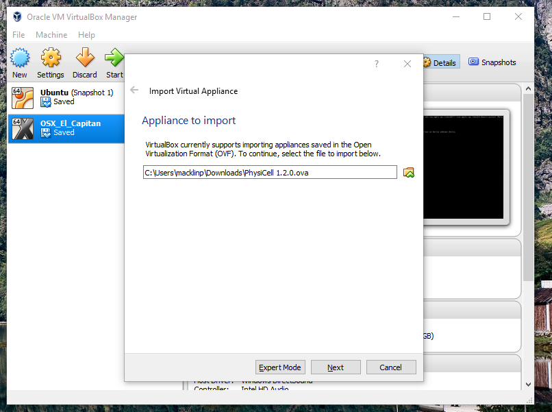
Click on “Next,” and import with all the default options. That’s it!
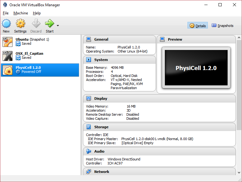
3) [Optional] Change settings
You most likely won’t need this step, but you can increase/decrease the amount of RAM used for the virtual machine if you select the PhysiCell VM, click the Settings button (orange gear), and choose “System”: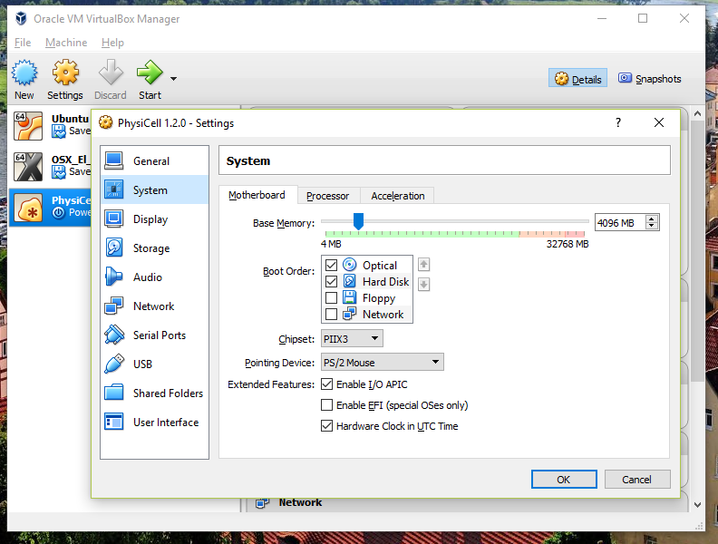 We set the Virtual Machine to have 4 GB of RAM. If you have a machine with lots of RAM (16 GB or more), you may want to set this to 8 GB.
Also, you can choose how many virtual CPUs to give to your VM: 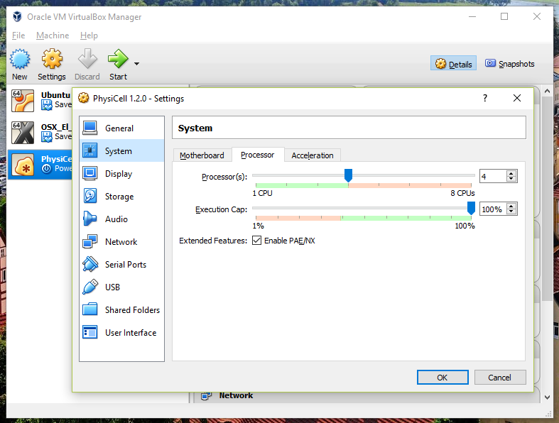
We selected 4 when we set up the Virtual Appliance, but you should match the number of physical processor cores on your machine. In my case, I have a quad core processor with hyperthreading. This means 4 real cores, 8 virtual cores, so I select 4 here.
4) Start the Virtual Machine and log in
Select the PhysiCell machine, and click the green “start” button. After the virtual machine boots (with the good old LILO boot manager that I’ve missed), you should see this:
Click the "More ..." button, and log in with username: physicell, password: physicell
5) Test the compiler and run your first simulation
Notice that PhysiCell is already there on the desktop in the PhysiCell folder. Right-click, and choose “open terminal here.” You’ll already be in the main PhysiCell root directory. 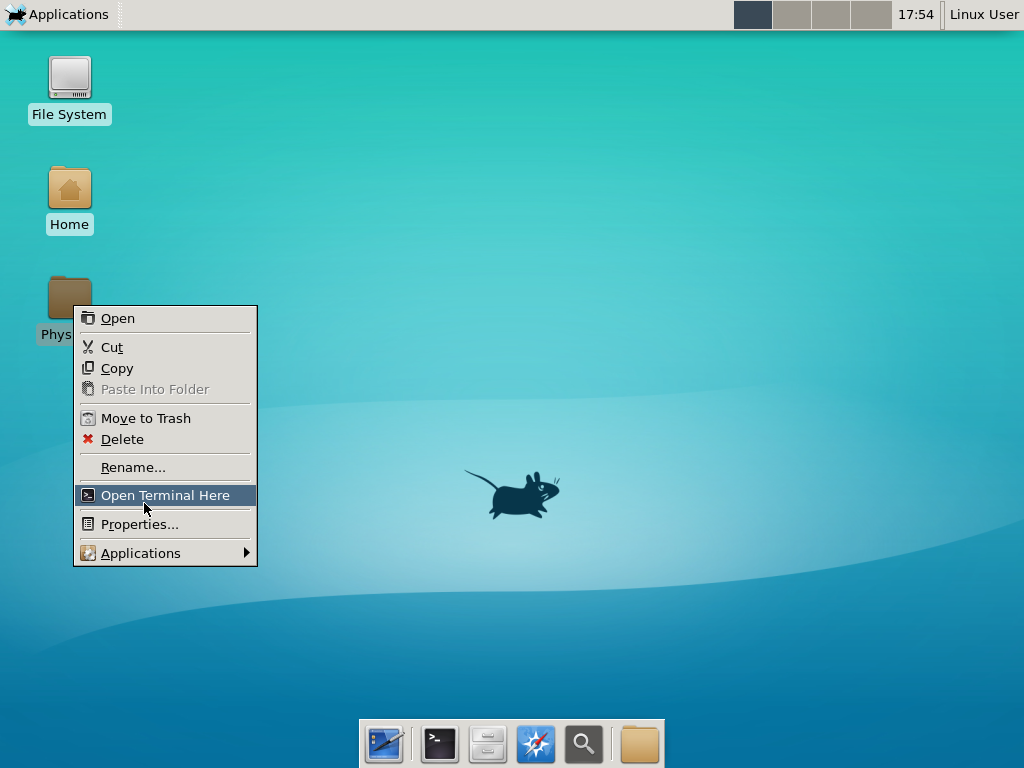
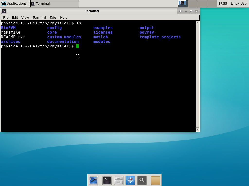
Now, let’s compile your first project! Type “make template2D && make” 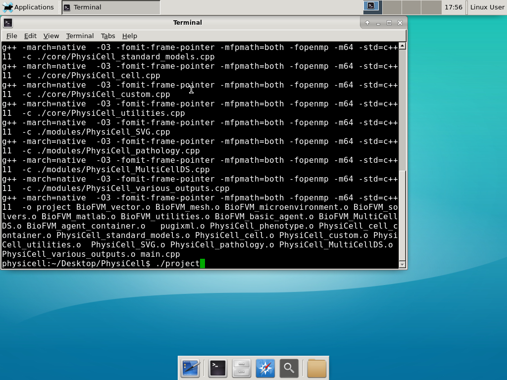 And run your project! Type “./project” and let it go!
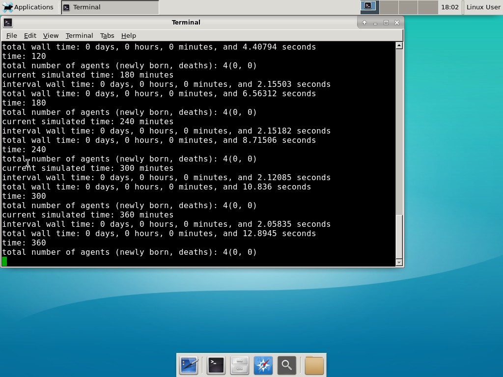 Go ahead and run either the first few days of the simulation (until about 7200 minutes), then hit <control>-C to cancel out. Or run the whole simulation–that’s fine, too.
6) Look at the results
We bundled a few tools to easily look at results. First, ristretto is a very fast image viewer. Let’s view the SVG files: 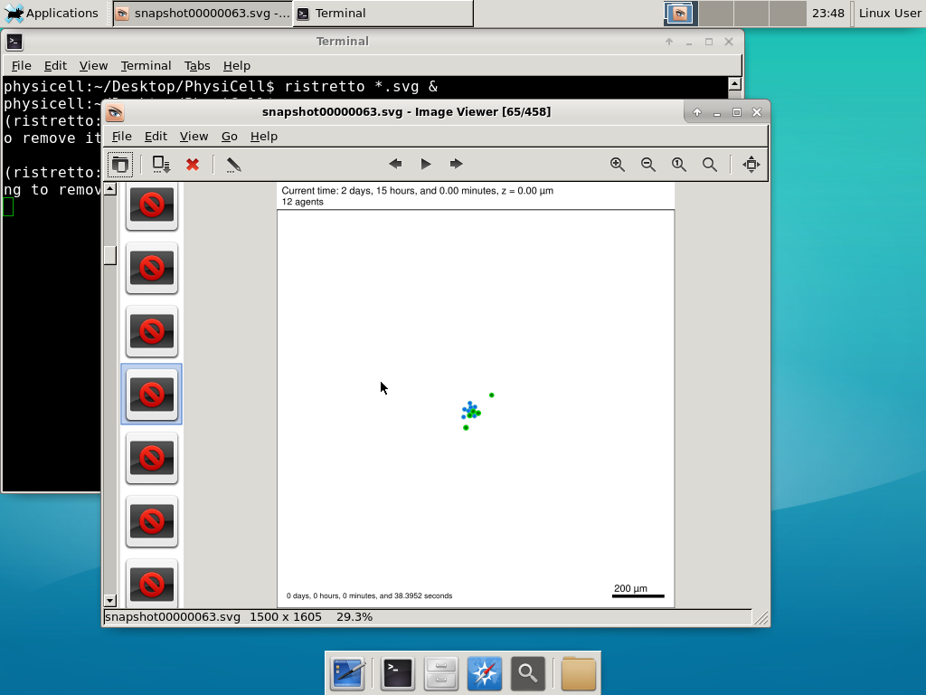 As a nice tip, you can press the left and right arrows to advance through the SVG images, or hold the right arrow down to advance through quickly.
Now, let’s use ImageMagick to convert the SVG files into JPG file: call “magick mogrify -format jpg snap*.svg”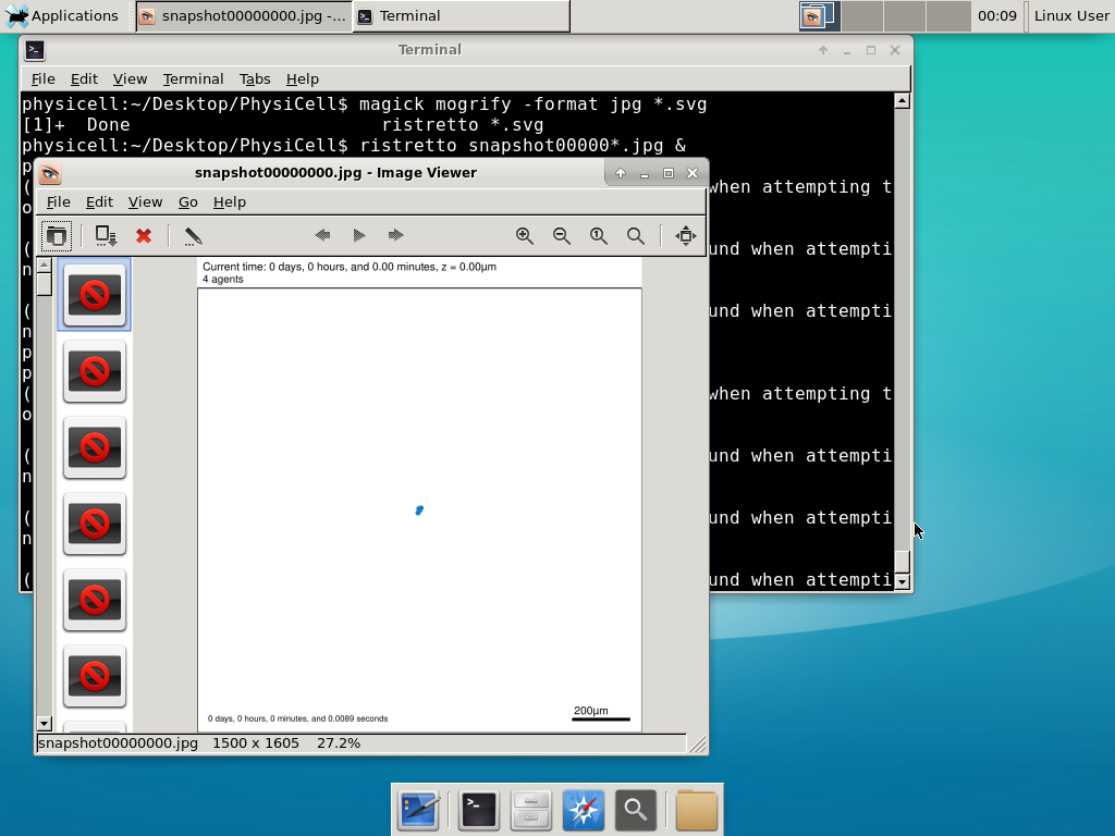
Next, let’s turn those images into a movie. I generally create moves that are 24 frames pers se, so that 1 second of the movie is 1 hour of simulations time. We’ll use mencoder, with options below given to help get a good quality vs. size tradeoff: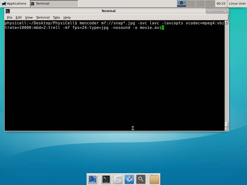
When you’re done, view the movie with mplayer. The options below scale the window to fit within the virtual monitor:
If you want to loop the movie, add “-loop 999” to your command.
7) Get familiar with other tools
Use nano (useage: nano <filename>) to quickly change files at the command line. Hit <control>-O to save your results. Hit <control>-X to exit. <control>-W will search within the file.
Use nedit (useage: nedit <filename> &) to open up one more text files in a graphical editor. This is a good way to edit multiple files at once.
Sometimes, you need to run commands at elevated (admin or root) privileges. Use sudo. Here’s an example, searching the Alpine Linux package manager apk for clang:
physicell:~$ sudo apk search gcc
[sudo] password for physicell:
physicell:~$ sudo apk search clang
clang-analyzer-4.0.0-r0
clang-libs-4.0.0-r0
clang-dev-4.0.0-r0
clang-static-4.0.0-r0
emscripten-fastcomp-1.37.10-r0
clang-doc-4.0.0-r0
clang-4.0.0-r0
physicell:~/Desktop/PhysiCell$
If you want to install clang/llvm (as an alternative compiler):
physicell:~$ sudo apk add gcc
[sudo] password for physicell:
physicell:~$ sudo apk search clang
clang-analyzer-4.0.0-r0
clang-libs-4.0.0-r0
clang-dev-4.0.0-r0
clang-static-4.0.0-r0
emscripten-fastcomp-1.37.10-r0
clang-doc-4.0.0-r0
clang-4.0.0-r0
physicell:~/Desktop/PhysiCell$
Notice that it asks for a password: use the password for root (which is physicell).
8) [Optional] Configure a shared folder
Coming soon.
Why both with zipped source, then?
Given that we can get a whole development environment by just downloading and importing a virtual appliance, why
bother with all the setup of a native development environment, like this tutorial (Windows) or this tutorial (Mac)?
One word: performance. In my testing, I still have not found the performance running inside a
virtual machine to match compiling and running directly on your system. So, the Virtual Appliance is a great
option to get up and running quickly while trying things out, but I still recommend setting up natively with
one of the tutorials I linked in the preceding paragraphs.
What’s next?
In the coming weeks, we’ll post further tutorials on using PhysiCell. In the meantime, have a look at the
PhysiCell project website, and these links as well:
- BioFVM on MathCancer.org: http://BioFVM.MathCancer.org
- BioFVM on SourceForge: http://BioFVM.sf.net
- BioFVM Method Paper in BioInformatics: http://dx.doi.org/10.1093/bioinformatics/btv730
- PhysiCell on MathCancer.org: http://PhysiCell.MathCancer.org
- PhysiCell on Sourceforge: http://PhysiCell.sf.net
- PhysiCell Method Paper (preprint): https://doi.org/10.1101/088773
- PhysiCell tutorials: [click here]
Coarse-graining discrete cell cycle models
Introduction
One observation that often goes underappreciated in computational biology discussions is that a computational model is often a model of a model of a model of biology: that is, it’s a numerical approximation (a model) of a mathematical model of an experimental model of a real-life biological system. Thus, there are three big places where a computational investigation can fall flat:
- The experimental model may be a bad choice for the disease or process (not our fault).
- Second, the mathematical model of the experimental system may have flawed assumptions (something we have to evaluate).
- The numerical implementation may have bugs or otherwise be mathematically inconsistent with the mathematical model.
Critically, you can’t use simulations to evaluate the experimental model or the mathematical model until you verify that the numerical implementation is consistent with the mathematical model, and that the numerical solution converges as \( \Delta t\) and \( \Delta x \) shrink to zero.
There are numerous ways to accomplish this, but ideally, it boils down to having some analytical solutions to the mathematical model, and comparing numerical solutions to these analytical or theoretical results. In this post, we’re going to walk through the math of analyzing a typical type of discrete cell cycle model.
Discrete model
Suppose we have a cell cycle model consisting of phases \(P_1, P_2, \ldots P_n \), where cells in the \(P_i\) phase progress to the \(P_{i+1}\) phase after a mean waiting time of \(T_i\), and cells leaving the \(P_n\) phase divide into two cells in the \(P_1\) phase. Assign each cell agent \(k\) a current phenotypic phase \( S_k(t) \). Suppose also that each phase \( i \) has a death rate \( d_i \), and that cells persist for on average \( T_\mathrm{A} \) time in the dead state before they are removed from the simulation.
The mean waiting times \( T_i \) are equivalent to transition rates \( r_i = 1 / T_i \) (Macklin et al. 2012). Moreover, for any time interval \( [t,t+\Delta t] \), both are equivalent to a transition probability of
\[ \mathrm{Prob}\Bigl( S_k(t+\Delta t) = P_{i+1} | S(t) = P_i \Bigr) = 1 – e^{ -r_i \Delta t } \approx r_i \Delta t = \frac{ \Delta t}{ T_i}. \] In many discrete models (especially cellular automaton models) with fixed step sizes \( \Delta t \), models are stated in terms of transition probabilities \( p_{i,i+1} \), which we see are equivalent to the work above with \( p_{i,i+1} = r_i \Delta t = \Delta t / T_i \), allowing us to tie mathematical model forms to biological, measurable parameters. We note that each \(T_i\) is the average duration of the \( P_i \) phase.
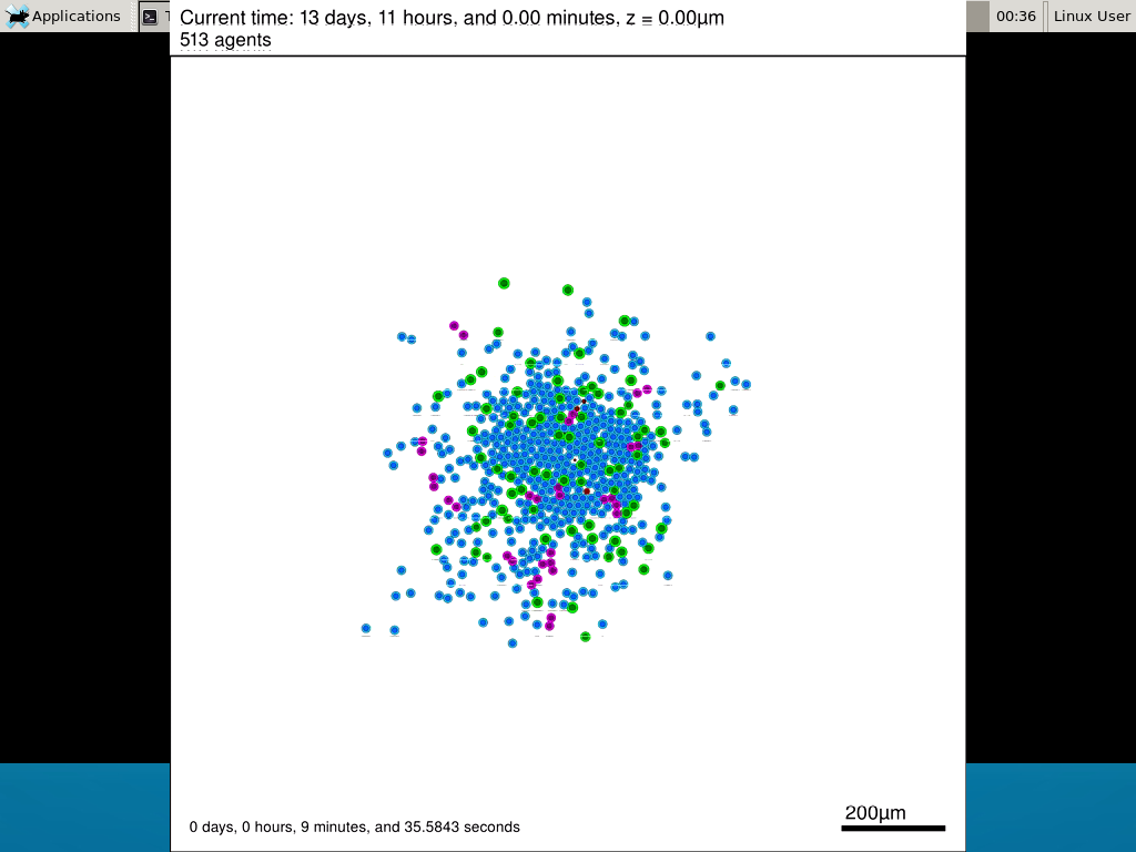
Concrete example: a Ki67 Model
Ki-67 is a nuclear protein that is expressed through much of the cell cycle, including S, G2, M, and part of G1 after division. It is used very commonly in pathology to assess proliferation, particularly in cancer. See the references and discussion in (Macklin et al. 2012). In Macklin et al. (2012), we came up with a discrete cell cycle model to match Ki-67 data (along with cleaved Caspase-3 stains for apoptotic cells). Let’s summarize the key parts here.
Each cell agent \(i\) has a phase \(S_i(t)\). Ki67- cells are quiescent (phase \(Q\), mean duration \( T_\mathrm{Q} \)), and they can enter the Ki67+ \(K_1\) phase (mean duration \(T_1\)). When \( K_1 \) cells leave their phase, they divide into two Ki67+ daughter cells in the \( K_2 \) phase with mean duration \( T_2 \). When cells exit \( K_2 \), they return to \( Q \). Cells in any phase can become apoptotic (enter the \( A \) phase with mean duration \( T_\mathrm{A} \)), with death rate \( r_\mathrm{A} \).
Coarse-graining to an ODE model
If each phase \(i\) has a death rate \(d_i\), if \( N_i(t) \) denotes the number of cells in the \( P_i \) phase at time \( t\), and if \( A(t) \) is the number of dead (apoptotic) cells at time \( t\), then on average, the number of cells in the \( P_i \) phase at the next time step is given by
\[ N_i(t+\Delta t) = N_i(t) + N_{i-1}(t) \cdot \left[ \textrm{prob. of } P_{i-1} \rightarrow P_i \textrm{ transition} \right] – N_i(t) \cdot \left[ \textrm{prob. of } P_{i} \rightarrow P_{i+1} \textrm{ transition} \right] \] \[ – N_i(t) \cdot \left[ \textrm{probability of death} \right] \] By the work above, this is:
\[ N_i(t+\Delta t) \approx N_i(t) + N_{i-1}(t) r_{i-1} \Delta t – N_i(t) r_i \Delta t – N_i(t) d_i \Delta t , \] or after shuffling terms and taking the limit as \( \Delta t \downarrow 0\), \[ \frac{d}{dt} N_i(t) = r_{i-1} N_{i-1}(t) – \left( r_i + d_i \right) N_i(t). \] Continuing this analysis, we obtain a linear system:
\[ \frac{d}{dt}{ \vec{N} } = \begin{bmatrix} -(r_1+d_1) & 0 & \cdots & 0 & 2r_n & 0 \\ r_1 & -(r_2+d_2) & 0 & \cdots & 0 & 0 \\ 0 & r_2 & -(r_3+d_3) & 0 & \cdots & 0 \\ & & \ddots & & \\0&\cdots&0 &r_{n-1} & -(r_n+d_n) & 0 \\ d_1 & d_2 & \cdots & d_{n-1} & d_n & -\frac{1}{T_\mathrm{A}} \end{bmatrix}\vec{N} = M \vec{N}, \] where \( \vec{N}(t) = [ N_1(t), N_2(t) , \ldots , N_n(t) , A(t) ] \).
For the Ki67 model above, let \(\vec{N} = [K_1, K_2, Q, A]\). Then the linear system is
\[ \frac{d}{dt} \vec{N} = \begin{bmatrix} -\left( \frac{1}{T_1} + r_\mathrm{A} \right) & 0 & \frac{1}{T_\mathrm{Q}} & 0 \\ \frac{2}{T_1} & -\left( \frac{1}{T_2} + r_\mathrm{A} \right) & 0 & 0 \\ 0 & \frac{1}{T_2} & -\left( \frac{1}{T_\mathrm{Q}} + r_\mathrm{A} \right) & 0 \\ r_\mathrm{A} & r_\mathrm{A} & r_\mathrm{A} & -\frac{1}{T_\mathrm{A}} \end{bmatrix} \vec{N} .\]
(If we had written \( \vec{N} = [Q, K_1, K_2 , A] \), then the matrix above would have matched the general form.)
Some theoretical results
If \( M\) has eigenvalues \( \lambda_1 , \ldots \lambda_{n+1} \) and corresponding eigenvectors \( \vec{v}_1, \ldots , \vec{v}_{n+1} \), then the general solution is given by
\[ \vec{N}(t) = \sum_{i=1}^{n+1} c_i e^{ \lambda_i t } \vec{v}_i ,\] and if the initial cell counts are given by \( \vec{N}(0) \) and we write \( \vec{c} = [c_1, \ldots c_{n+1} ] \), we can obtain the coefficients by solving \[ \vec{N}(0) = [ \vec{v}_1 | \cdots | \vec{v}_{n+1} ]\vec{c} .\] In many cases, it turns out that all but one of the eigenvalues (say \( \lambda \) with corresponding eigenvector \(\vec{v}\)) are negative. In this case, all the other components of the solution decay away, and for long times, we have \[ \vec{N}(t) \approx c e^{ \lambda t } \vec{v} .\] This is incredibly useful, because it says that over long times, the fraction of cells in the \( i^\textrm{th} \) phase is given by \[ v_{i} / \sum_{j=1}^{n+1} v_{j}. \]
Matlab implementation (with the Ki67 model)
First, let’s set some parameters, to make this a little easier and reusable.
parameters.dt = 0.1; % 6 min = 0.1 hours
parameters.time_units = 'hour';
parameters.t_max = 3*24; % 3 days

parameters.K1.duration =  13;
parameters.K1.death_rate = 1.05e-3;
parameters.K1.initial = 0;

parameters.K2.duration = 2.5;
parameters.K2.death_rate = 1.05e-3;
parameters.K2.initial = 0;

parameters.Q.duration = 74.35 ;
parameters.Q.death_rate = 1.05e-3;
parameters.Q.initial = 1000;

parameters.A.duration = 8.6;
parameters.A.initial = 0;
Next, we write a function to read in the parameter values, construct the matrix (and all the data structures), find eigenvalues and eigenvectors, and create the theoretical solution. It also finds the positive eigenvalue to determine the long-time values.
function solution = Ki67_exact( parameters )
% allocate memory for the main outputs
solution.T = 0:parameters.dt:parameters.t_max;
solution.K1 = zeros( 1 , length(solution.T));
solution.K2 = zeros( 1 , length(solution.T));
solution.K = zeros( 1 , length(solution.T));
solution.Q = zeros( 1 , length(solution.T));
solution.A = zeros( 1 , length(solution.T));
solution.Live = zeros( 1 , length(solution.T));
solution.Total = zeros( 1 , length(solution.T));
% allocate memory for cell fractions
solution.AI = zeros(1,length(solution.T));
solution.KI1 = zeros(1,length(solution.T));
solution.KI2 = zeros(1,length(solution.T));
solution.KI = zeros(1,length(solution.T));
% get the main parameters
T1 = parameters.K1.duration;
r1A = parameters.K1.death_rate;
T2 = parameters.K2.duration;
r2A = parameters.K2.death_rate;
TQ = parameters.Q.duration;
rQA = parameters.Q.death_rate;
TA = parameters.A.duration;
% write out the mathematical model:
% d[Populations]/dt = Operator*[Populations]
Operator = [ -(1/T1 +r1A) , 0 , 1/TQ , 0; ...
2/T1 , -(1/T2 + r2A) ,0 , 0; ...
0 , 1/T2 , -(1/TQ + rQA) , 0; ...
r1A , r2A, rQA , -1/TA ];
% eigenvectors and eigenvalues
[V,D] = eig(Operator);
eigenvalues = diag(D);
% save the eigenvectors and eigenvalues in case you want them.
solution.V = V;
solution.D = D;
solution.eigenvalues = eigenvalues;
% initial condition
VecNow = [ parameters.K1.initial ; parameters.K2.initial ; ...
parameters.Q.initial ; parameters.A.initial ] ;
solution.K1(1) = VecNow(1);
solution.K2(1) = VecNow(2);
solution.Q(1) = VecNow(3);
solution.A(1) = VecNow(4);
solution.K(1) = solution.K1(1) + solution.K2(1);
solution.Live(1) = sum( VecNow(1:3) );
solution.Total(1) = sum( VecNow(1:4) );
solution.AI(1) = solution.A(1) / solution.Total(1);
solution.KI1(1) = solution.K1(1) / solution.Total(1);
solution.KI2(1) = solution.K2(1) / solution.Total(1);
solution.KI(1) = solution.KI1(1) + solution.KI2(1);
% now, get the coefficients to write the analytic solution
% [Populations] = c1*V(:,1)*exp( d(1,1)*t) + c2*V(:,2)*exp( d(2,2)*t ) +
% c3*V(:,3)*exp( d(3,3)*t) + c4*V(:,4)*exp( d(4,4)*t );
coeff = linsolve( V , VecNow );
% find the (hopefully one) positive eigenvalue.
% eigensolutions with negative eigenvalues decay,
% leaving this as the long-time behavior.
eigenvalues = diag(D);
n = find( real( eigenvalues ) &gt; 0 )
solution.long_time.KI1 = V(1,n) / sum( V(:,n) );
solution.long_time.KI2 = V(2,n) / sum( V(:,n) );
solution.long_time.QI = V(3,n) / sum( V(:,n) );
solution.long_time.AI = V(4,n) / sum( V(:,n) ) ;
solution.long_time.KI = solution.long_time.KI1 + solution.long_time.KI2;
% now, write out the solution at all the times
for i=2:length( solution.T )
% compact way to write the solution
VecExact = real( V*( coeff .* exp( eigenvalues*solution.T(i) ) ) );
solution.K1(i) = VecExact(1);
solution.K2(i) = VecExact(2);
solution.Q(i) = VecExact(3);
solution.A(i) = VecExact(4);
solution.K(i) = solution.K1(i) + solution.K2(i);
solution.Live(i) = sum( VecExact(1:3) );
solution.Total(i) = sum( VecExact(1:4) );
solution.AI(i) = solution.A(i) / solution.Total(i);
solution.KI1(i) = solution.K1(i) / solution.Total(i);
solution.KI2(i) = solution.K2(i) / solution.Total(i);
solution.KI(i) = solution.KI1(i) + solution.KI2(i);
end
return;
Now, let’s run it and see what this thing looks like:
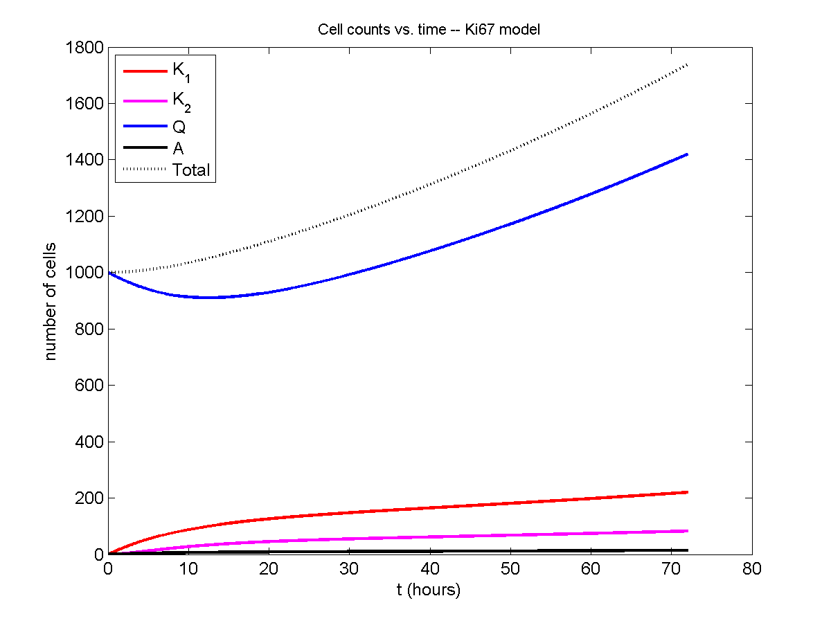
Next, we plot KI1, KI2, and AI versus time (solid curves), along with the theoretical long-time behavior (dashed curves). Notice how well it matches–it’s neat when theory works! :-)
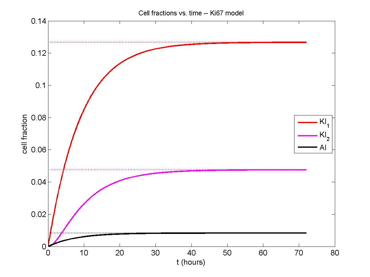
Some readers may recognize the long-time fractions: KI1 + KI2 = KI = 0.1743, and AI = 0.00833, very close to the DCIS patient values from our simulation study in Macklin et al. (2012) and improved calibration work in Hyun and Macklin (2013).
Comparing simulations and theory
I wrote a small Matlab program to implement the discrete model: start with 1000 cells in the \(Q\) phase, and in each time interval \([t,t+\Delta t]\), each cell “decides” whether to advance to the next phase, stay in the same phase, or apoptose. If we compare a single run against the theoretical curves, we see hints of a match:
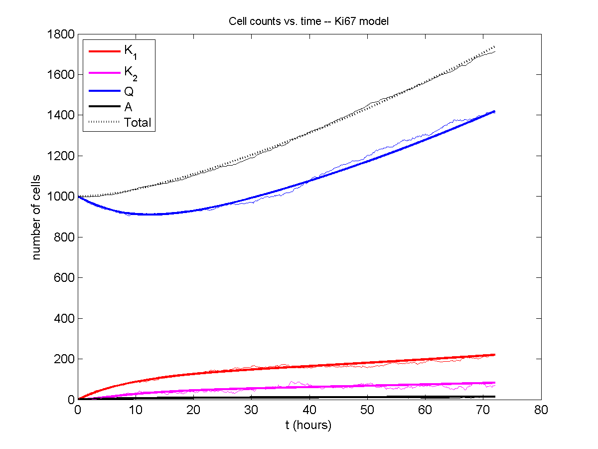
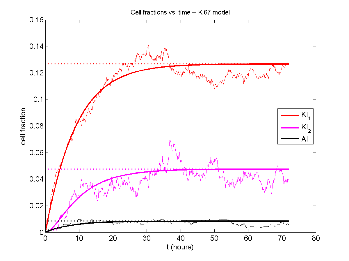
If we average 10 simulations and compare, the match is better:

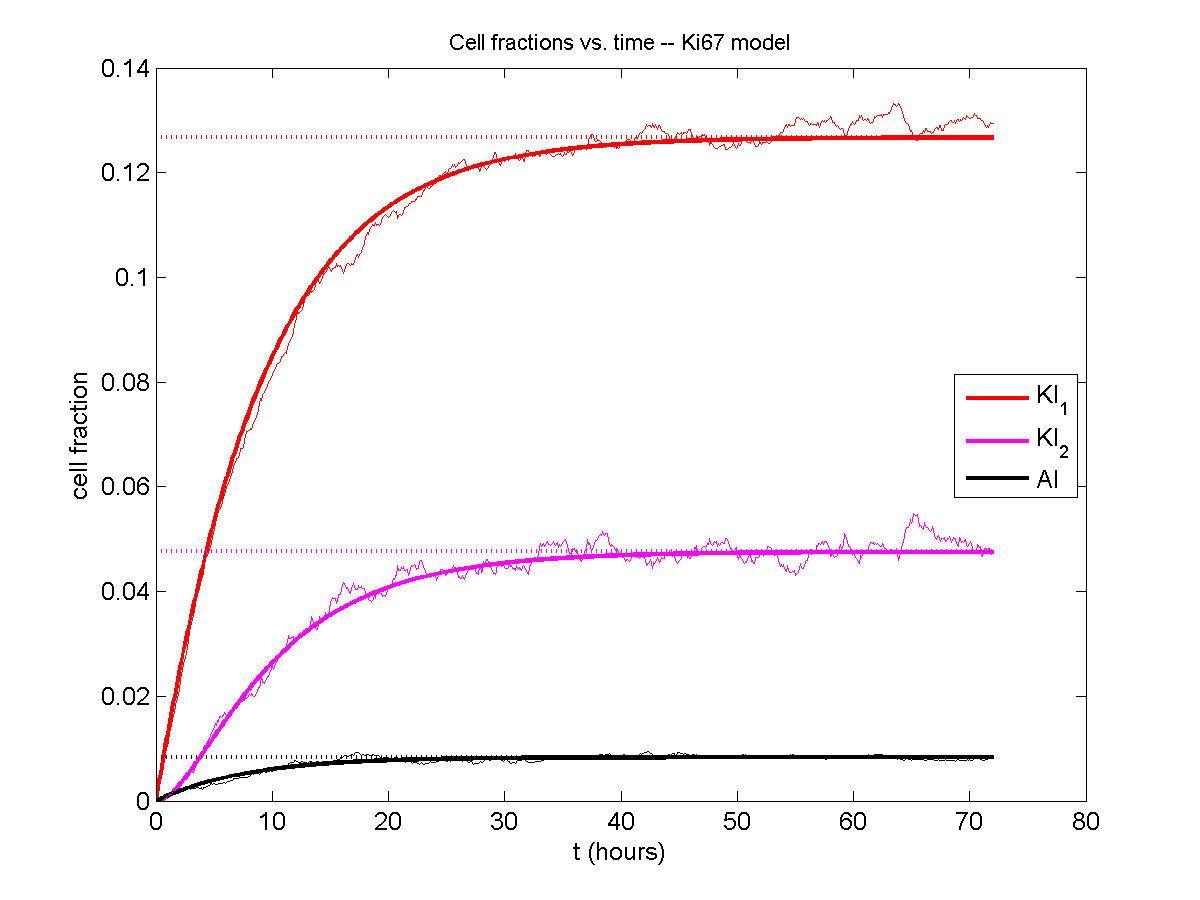
And lastly, if we average 100 simulations and compare, the curves are very difficult to tell apart:
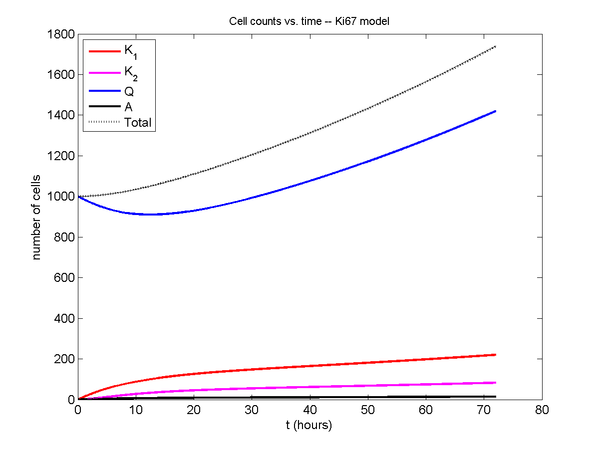

Even in logarithmic space, it’s tough to tell these apart:
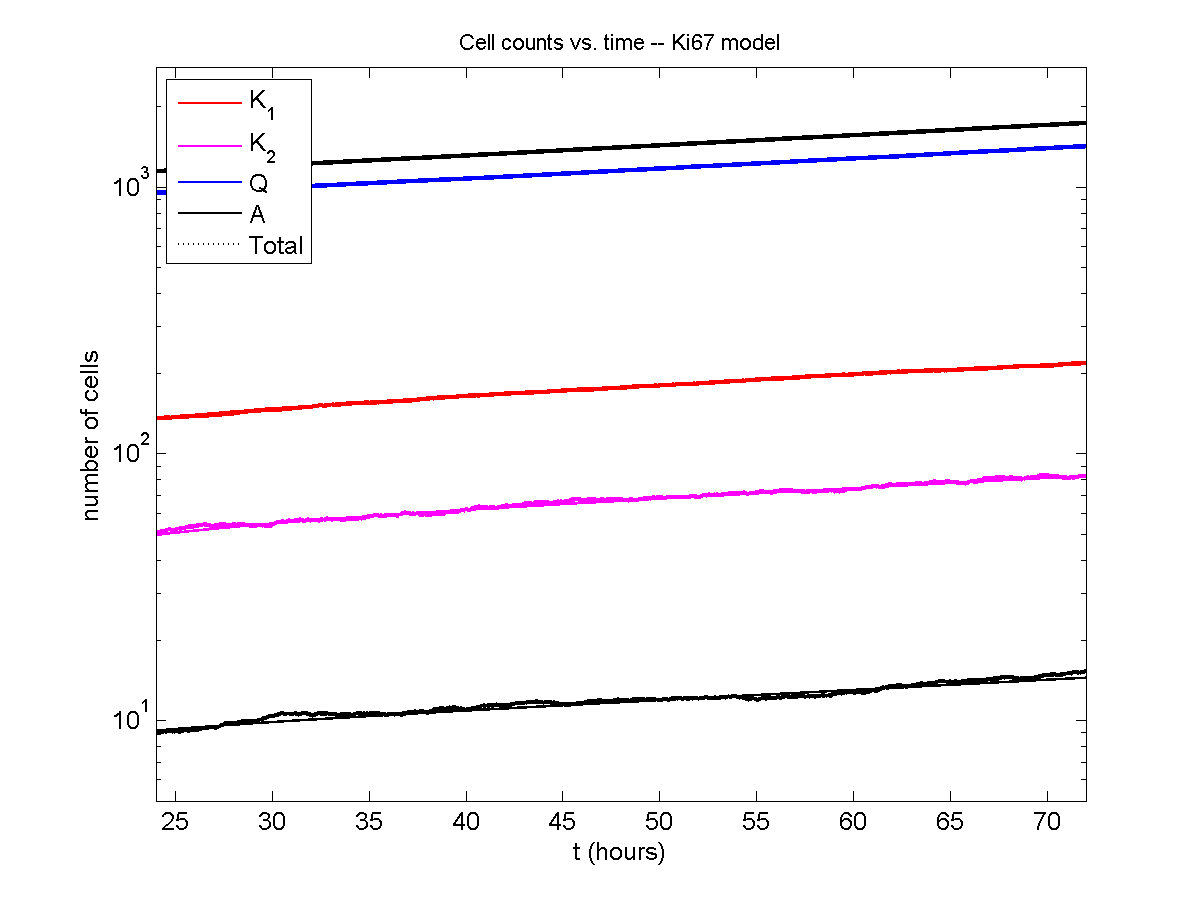
Code
The following matlab files (available here) can be used to reproduce this post:
- Ki67_exact.m
- The function defined above to create the exact solution using the eigenvalue/eignvector approach.
- Ki67_stochastic.m
- Runs a single stochastic simulation, using the supplied parameters.
- script.m
- Runs the theoretical solution first, creates plots, and then runs the stochastic model 100 times for comparison.
To make it all work, simply run “script” at the command prompt. Please note that it will generate some png files in its directory.
Closing thoughts
In this post, we showed a nice way to check a discrete model against theoretical behavior–both in short-term dynamics and long-time behavior. The same work should apply to validating many discrete models. However, when you add spatial effects (e.g., a cellular automaton model that won’t proliferate without an empty neighbor site), I wouldn’t expect a match. (But simulating cells that initially have a “salt and pepper”, random distribution should match this for early times.)
Moreover, models with deterministic phase durations (e.g., K1, K2, and A have fixed durations) aren’t consistent with the ODE model above, unless the cells they are each initialized with a random amount of “progress” in their initial phases. (Otherwise, the cells in each phase will run synchronized, and there will be fixed delays before cells transition to other phases.) Delay differential equations better describe such models. However, for long simulation times, the slopes of the sub-populations and the cell fractions should start to better and better match the ODE models.
Now that we have verified that the discrete model is performing as expected, we can have greater confidence in its predictions, and start using those predictions to assess the underlying models. In ODE and PDE models, you often validate the code on simpler problems where you have an analytical solution, and then move on to making simulation predictions in cases where you can’t solve analytically. Similarly, we can now move on to variants of the discrete model where we can’t as easily match ODE theory (e.g., time-varying rate parameters, spatial effects), but with the confidence that the phase transitions are working as they should.
Building a Cellular Automaton Model Using BioFVM
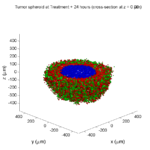
Note: This is part of a series of “how-to” blog posts to help new users and developers of BioFVM. See below for guides to setting up a C++ compiler in Windows or OSX.
What you’ll need
- A working C++ development environment with support for OpenMP. See these prior tutorials if you need help.
- A download of BioFVM, available at http://BioFVM.MathCancer.org and http://BioFVM.sf.net. Use Version 1.1.4 or later.
- The source code for this project (see below).
Matlab or Octave for visualization. Matlab might be available for free at your university. Octave is open source and available from a variety of sources.
Our modeling task
We will implement a basic 3-D cellular automaton model of tumor growth in a well-mixed fluid, containing oxygen pO2 (mmHg) and a drug c (e.g., doxorubicin, μM), inspired by modeling by Alexander Anderson, Heiko Enderling, Jan Poleszczuk, Gibin Powathil, and others. (I highly suggest seeking out the sophisticated cellular automaton models at Moffitt’s Integrated Mathematical Oncology program!) This example shows you how to extend BioFVM into a new cellular automaton model. I’ll write a similar post on how to add BioFVM into an existing cellular automaton model, which you may already have available.
Tumor growth will be driven by oxygen availability. Tumor cells can be live, apoptotic (going through energy-dependent cell death, or necrotic (undergoing death from energy collapse). Drug exposure can both trigger apoptosis and inhibit cell cycling. We will model this as growth into a well-mixed fluid, with pO2 = 38 mmHg (about 5% oxygen: a physioxic value) and c = 5 μM.
Mathematical model
As a cellular automaton model, we will divide 3-D space into a regular lattice of voxels, with length, width, and height of 15 μm. (A typical breast cancer cell has radius around 9-10 μm, giving a typical volume around 3.6×103 μm3. If we make each lattice site have the volume of one cell, this gives an edge length around 15 μm.)
In voxels unoccupied by cells, we approximate a well-mixed fluid with Dirichlet nodes, setting pO2 = 38 mmHg, and initially setting c = 0. Whenever a cell dies, we replace it with an empty automaton, with no Dirichlet node. Oxygen and drug follow the typical diffusion-reaction equations:
\[ \frac{ \partial \textrm{pO}_2 }{\partial t} = D_\textrm{oxy} \nabla^2 \textrm{pO}_2 – \lambda_\textrm{oxy} \textrm{pO}_2 – \sum_{ \textrm{cells} i} U_{i,\textrm{oxy}} \textrm{pO}_2 \]
\[ \frac{ \partial c}{ \partial t } = D_c \nabla^2 c – \lambda_c c – \sum_{\textrm{cells }i} U_{i,c} c \]
where each uptake rate is applied across the cell’s volume. We start the treatment by setting c = 5 μM on all Dirichlet nodes at t = 504 hours (21 days). For simplicity, we do not model drug degradation (pharmacokinetics), to approximate the in vitro conditions.
In any time interval [t,t+Δt], each live tumor cell i has a probability pi,D of attempting division, probability pi,A of apoptotic death, and probability pi,N of necrotic death. (For simplicity, we ignore motility in this version.) We relate these to the birth rate bi, apoptotic death rate di,A, and necrotic death rate di,N by the linearized equations (from Macklin et al. 2012):
\[ \textrm{Prob} \Bigl( \textrm{cell } i \textrm{ becomes apoptotic in } [t,t+\Delta t] \Bigr) = 1 – \textrm{exp}\Bigl( -d_{i,A}(t) \Delta t\Bigr) \approx d_{i,A}\Delta t \]
\[ \textrm{Prob} \Bigl( \textrm{cell } i \textrm{ attempts division in } [t,t+\Delta t] \Bigr) = 1 – \textrm{exp}\Bigl( -b_i(t) \Delta t\Bigr) \approx b_{i}\Delta t \]
\[ \textrm{Prob} \Bigl( \textrm{cell } i \textrm{ becomes necrotic in } [t,t+\Delta t] \Bigr) = 1 – \textrm{exp}\Bigl( -d_{i,N}(t) \Delta t\Bigr) \approx d_{i,N}\Delta t \]
\[ \textrm{Prob} \Bigl( \textrm{dead cell } i \textrm{ lyses in } [t,t+\Delta t] \Bigr) = 1 – \textrm{exp}\Bigl( -\frac{1}{T_{i,D}} \Delta t\Bigr) \approx \frac{ \Delta t}{T_{i,D}} \]
(Illustrative) parameter values
We use Doxy = 105 μm2/min (Ghaffarizadeh et al. 2016), and we set Ui,oxy = 20 min-1 (to give an oxygen diffusion length scale of about 70 μm, with steeper gradients than our typical 100 μm length scale). We set λoxy = 0.01 min-1 for a 1 mm diffusion length scale in fluid.
We set Dc = 300 μm2/min, and Uc = 7.2×10⁻³ min-1 (Dc from Weinberg et al. (2007), and Ui,c twice as large as the reference value in Weinberg et al. (2007) to get a smaller diffusion length scale of about 204 μm). We set λc = 3.6×10⁻⁵ min-1 to give a drug diffusion length scale of about 2.9 mm in fluid.
We use TD = 8.6 hours for apoptotic cells, and TD = 60 days for necrotic cells (Macklin et al., 2013). However, note that necrotic and apoptotic cells lose volume quickly, so one may want to revise those time scales to match the point where a cell loses 90% of its volume.
Functional forms for the birth and death rates
We model pharmacodynamics with an area-under-the-curve (AUC) type formulation. If c(t) is the drug concentration at any cell i‘s location at time t, then let its integrated exposure Ei(t) be
\[ E_i(t) = \int_0^t c(s) \: ds \]
and we model its response with a Hill function
\[ R_i(t) = \frac{ E_i^h(t) }{ \alpha_i^h + E_i^h(t) }, \]
where h is the drug’s Hill exponent for the cell line, and α is the exposure for a half-maximum effect.
We model the microenvironment-dependent birth rate by:
\[ b_i(t) = \left\{ \begin{array}{lr} b_{i,P} \left( 1 – \eta_i R_i(t) \right) & \textrm{ if } \textrm{pO}_{2,P} < \textrm{pO}_2 \\ \\ b_{i,P} \left( \frac{\textrm{pO}_{2}-\textrm{pO}_{2,N}}{\textrm{pO}_{2,P}-\textrm{pO}_{2,N}}\right) \Bigl( 1 – \eta_i R_i(t) \Bigr) & \textrm{ if } \textrm{pO}_{2,N} < \textrm{pO}_2 \le \textrm{pO}_{2,P} \\ \\ 0 & \textrm{ if } \textrm{pO}_2 \le \textrm{pO}_{2,N}\end{array} \right. \]
where pO2,P is the physioxic oxygen value (38 mmHg), and pO2,N is a necrotic threshold (we use 5 mmHg), and 0 < η < 1 the drug’s birth inhibition. (A fully cytostatic drug has η = 1.)
We model the microenvironment-dependent apoptosis rate by:
\[ d_{i,A}(t) = d_{i,A}^* + \Bigl( d_{i,A}^\textrm{max} – d_{i,A}^* \Bigr) R_i(t) \]
\[ d_{i,N}(t) = \left\{ \begin{array}{lr} 0 & \textrm{ if } \textrm{pO}_{2,N} < \textrm{pO}_{2} \\ \\ d_{i,N}^* & \textrm{ if } \textrm{pO}_{2} \le \textrm{pO}_{2,N} \end{array}\right. \]
(Illustrative) parameter values
We use bi,P = 0.05 hour-1 (for a 20 hour cell cycle in physioxic conditions), di,A* = 0.01 bi,P, and di,N* = 0.04 hour-1 (so necrotic cells survive around 25 hours in low oxygen conditions).
We set α = 30 μM*hour (so that cells reach half max response after 6 hours’ exposure at a maximum concentration c = 5 μM), h = 2 (for a smooth effect), η = 0.25 (so that the drug is partly cytostatic), and di,Amax = 0.1 hour^-1 (so that cells survive about 10 hours after reaching maximum response).
Building the Cellular Automaton Model in BioFVM
BioFVM already includes Basic_Agents for cell-based substrate sources and sinks. We can extend these basic agents into full-fledged automata, and then arrange them in a lattice to create a full cellular automata model. Let’s sketch that out now.
Extending Basic_Agents to Automata
The main idea here is to define an Automaton class which extends (and therefore includes) the Basic_Agent class. This will give each Automaton full access to the microenvironment defined in BioFVM, including the ability to secrete and uptake substrates. We also make sure each Automaton “knows” which microenvironment it lives in (contains a pointer pMicroenvironment), and “knows” where it lives in the cellular automaton lattice. (More on that in the following paragraphs.)
So, as a schematic (just sketching out the most important members of the class):
class Standard_Data; // define per-cell biological data, such as phenotype,
	// cell cycle status, etc..
class Custom_Data; // user-defined custom data, specific to a model.

class Automaton : public Basic_Agent
{
	private:
		Microenvironment* pMicroenvironment;

		CA_Mesh* pCA_mesh;
		int voxel_index;

	protected:
	public:
		// neighbor connectivity information
		std::vector<Automaton*> neighbors;
		std::vector<double> neighbor_weights;

		Standard_Data standard_data;
		void (*current_state_rule)( Automaton& A , double );

		Automaton();
		void copy_parameters( Standard_Data& SD  );
		void overwrite_from_automaton( Automaton& A );

		void set_cellular_automaton_mesh( CA_Mesh* pMesh );
		CA_Mesh* get_cellular_automaton_mesh( void ) const;

		void set_voxel_index( int );
		int get_voxel_index( void ) const;

		void set_microenvironment( Microenvironment* pME );
		Microenvironment* get_microenvironment( void );

		// standard state changes
		bool attempt_division( void );
		void become_apoptotic( void );
		void become_necrotic( void );
		void perform_lysis( void );

		// things the user needs to define

		Custom_Data custom_data;

		// use this rule to add custom logic
		void (*custom_rule)( Automaton& A , double);
};
So, the Automaton class includes everything in the Basic_Agent class, some Standard_Data (things like the cell state and phenotype, and per-cell settings), (user-defined) Custom_Data, basic cell behaviors like attempting division into an empty neighbor lattice site, and user-defined custom logic that can be applied to any automaton. To avoid lots of switch/case and if/then logic, each Automaton has a function pointer for its current activity (current_state_rule), which can be overwritten any time.
Each Automaton also has a list of neighbor Automata (their memory addresses), and weights for each of these neighbors. Thus, you can distance-weight the neighbors (so that corner elements are farther away), and very generalized neighbor models are possible (e.g., all lattice sites within a certain distance). When updating a cellular automaton model, such as to kill a cell, divide it, or move it, you leave the neighbor information alone, and copy/edit the information (standard_data, custom_data, current_state_rule, custom_rule). In many ways, an Automaton is just a bucket with a cell’s information in it.
Note that each Automaton also “knows” where it lives (pMicroenvironment and voxel_index), and knows what CA_Mesh it is attached to (more below).
Connecting Automata into a Lattice
An automaton by itself is lost in the world–it needs to link up into a lattice organization. Here’s where we define a CA_Mesh class, to hold the entire collection of Automata, setup functions (to match to the microenvironment), and two fundamental operations at the mesh level: copying automata (for cell division), and swapping them (for motility). We have provided two functions to accomplish these tasks, while automatically keeping the indexing and BioFVM functions correctly in sync. Here’s what it looks like:
class CA_Mesh{
	private:
		Microenvironment* pMicroenvironment;
		Cartesian_Mesh* pMesh;

		std::vector<Automaton> automata;
		std::vector<int> iteration_order;
	protected:
	public:
		CA_Mesh();

		// setup to match a supplied microenvironment
		void setup( Microenvironment& M );
		// setup to match the default microenvironment
		void setup( void );

		int number_of_automata( void ) const;

		void randomize_iteration_order( void );

		void swap_automata( int i, int j );
		void overwrite_automaton( int source_i, int destination_i );

		// return the automaton sitting in the ith lattice site
		Automaton& operator[]( int i );

		// go through all nodes according to random shuffled order
		void update_automata( double dt );
};
So, the CA_Mesh has a vector of Automata (which are never themselves moved), pointers to the microenvironment and its mesh, and a vector of automata indices that gives the iteration order (so that we can sample the automata in a random order). You can easily access an automaton with operator[], and copy the data from one Automaton to another with overwrite_automaton() (e.g, for cell division), and swap two Automata’s data (e.g., for cell migration) with swap_automata(). Finally, calling update_automata(dt) iterates through all the automata according to iteration_order, calls their current_state_rules and custom_rules, and advances the automata by dt.
Interfacing Automata with the BioFVM Microenvironment
The setup function ensures that the CA_Mesh is the same size as the Microenvironment.mesh, with same indexing, and that all automata have the correct volume, and dimension of uptake/secretion rates and parameters. If you declare and set up the Microenvironment first, all this is take care of just by declaring a CA_Mesh, as it seeks out the default microenvironment and sizes itself accordingly:
// declare a microenvironment
Microenvironment M;
// do things to set it up -- see prior tutorials
// declare a Cellular_Automaton_Mesh
CA_Mesh CA_model;
// it's already good to go, initialized to empty automata:
CA_model.display();
If you for some reason declare the CA_Mesh fist, you can set it up against the microenvironment:
// declare a CA_Mesh
CA_Mesh CA_model;
// declare a microenvironment
Microenvironment M;
// do things to set it up -- see prior tutorials
// initialize the CA_Mesh to match the microenvironment
CA_model.setup( M );
// it's already good to go, initialized to empty automata:
CA_model.display();
Because each Automaton is in the microenvironment and inherits functions from Basic_Agent, it can secrete or uptake. For example, we can use functions like this one:
void set_uptake( Automaton& A, std::vector<double>& uptake_rates )
{
extern double BioFVM_CA_diffusion_dt;
// update the uptake_rates in the standard_data
A.standard_data.uptake_rates = uptake_rates;
// now, transfer them to the underlying Basic_Agent
*(A.uptake_rates) = A.standard_data.uptake_rates;
// and make sure the internal constants are self-consistent
A.set_internal_uptake_constants( BioFVM_CA_diffusion_dt );
}
A function acting on an automaton can sample the microenvironment to change parameters and state. For example:
void do_nothing( Automaton& A, double dt )
{ return; }

void microenvironment_based_rule( Automaton& A, double dt )
{
	// sample the microenvironment
	std::vector<double> MS = (*A.get_microenvironment())( A.get_voxel_index() );

	// if pO2 < 5 mmHg, set the cell to a necrotic state
	if( MS[0] < 5.0 ) { A.become_necrotic(); } // if drug > 5 uM, set the birth rate to zero
	if( MS[1] > 5 )
	{ A.standard_data.birth_rate = 0.0; }

	// set the custom rule to something else
	A.custom_rule = do_nothing;

	return;
}
Implementing the mathematical model in this framework
We give each tumor cell a tumor_cell_rule (using this for custom_rule):
void viable_tumor_rule( Automaton& A, double dt )
{
	// If there's no cell here, don't bother.
	if( A.standard_data.state_code == BioFVM_CA_empty )
	{ return; }

	// sample the microenvironment
	std::vector<double> MS = (*A.get_microenvironment())( A.get_voxel_index() );

	// integrate drug exposure
	A.standard_data.integrated_drug_exposure += ( MS[1]*dt );
	A.standard_data.drug_response_function_value = pow( A.standard_data.integrated_drug_exposure,
		A.standard_data.drug_hill_exponent );
	double temp = pow( A.standard_data.drug_half_max_drug_exposure,
		A.standard_data.drug_hill_exponent );
	temp += A.standard_data.drug_response_function_value;
	A.standard_data.drug_response_function_value /= temp;

	// update birth rates (which themselves update probabilities)
	update_birth_rate( A, MS, dt );
	update_apoptotic_death_rate( A, MS, dt );
	update_necrotic_death_rate( A, MS, dt );

	return;
}
The functional tumor birth and death rates are implemented as:
void update_birth_rate( Automaton& A, std::vector<double>& MS, double dt )
{
	static double O2_denominator = BioFVM_CA_physioxic_O2 - BioFVM_CA_necrotic_O2;

	A.standard_data.birth_rate = 	A.standard_data.drug_response_function_value;
		// response
	A.standard_data.birth_rate *= A.standard_data.drug_max_birth_inhibition;
		// inhibition*response;
	A.standard_data.birth_rate *= -1.0;
		// - inhibition*response
	A.standard_data.birth_rate += 1.0;
		// 1 - inhibition*response
	A.standard_data.birth_rate *= viable_tumor_cell.birth_rate;
		// birth_rate0*(1 - inhibition*response)

	double temp1 = MS[0] ; // O2
	temp1 -= BioFVM_CA_necrotic_O2;
	temp1 /= O2_denominator;

	A.standard_data.birth_rate *= temp1;
	if( A.standard_data.birth_rate < 0 )
	{ A.standard_data.birth_rate = 0.0; }

	A.standard_data.probability_of_division = A.standard_data.birth_rate;
	A.standard_data.probability_of_division *= dt;
		// dt*birth_rate*(1 - inhibition*repsonse) // linearized probability
	return;
}

void update_apoptotic_death_rate( Automaton& A, std::vector<double>& MS, double dt )
{
	A.standard_data.apoptotic_death_rate = A.standard_data.drug_max_death_rate;
		// max_rate
	A.standard_data.apoptotic_death_rate -= viable_tumor_cell.apoptotic_death_rate;
		// max_rate - background_rate
	A.standard_data.apoptotic_death_rate *= A.standard_data.drug_response_function_value;
		// (max_rate-background_rate)*response
	A.standard_data.apoptotic_death_rate += viable_tumor_cell.apoptotic_death_rate;
		// background_rate + (max_rate-background_rate)*response

	A.standard_data.probability_of_apoptotic_death = A.standard_data.apoptotic_death_rate;
	A.standard_data.probability_of_apoptotic_death *= dt;
		// dt*( background_rate + (max_rate-background_rate)*response ) // linearized probability
	return;
}

void update_necrotic_death_rate( Automaton& A, std::vector<double>& MS, double dt )
{
	A.standard_data.necrotic_death_rate = 0.0;
	A.standard_data.probability_of_necrotic_death = 0.0;

	if( MS[0] > BioFVM_CA_necrotic_O2 )
	{ return; }

	A.standard_data.necrotic_death_rate = perinecrotic_tumor_cell.necrotic_death_rate;
	A.standard_data.probability_of_necrotic_death = A.standard_data.necrotic_death_rate;
	A.standard_data.probability_of_necrotic_death *= dt;
		// dt*necrotic_death_rate

	return;
}
And each fluid voxel (Dirichlet nodes) is implemented as the following (to turn on therapy at 21 days):
void fluid_rule( Automaton& A, double dt )
{
	static double activation_time = 504;
	static double activation_dose = 5.0;
	static std::vector<double> activated_dirichlet( 2 , BioFVM_CA_physioxic_O2 );
	static bool initialized = false;
	if( !initialized )
	{
		activated_dirichlet[1] = activation_dose;
		initialized = true;
	}

	if( fabs( BioFVM_CA_elapsed_time - activation_time ) < 0.01 ) { int ind = A.get_voxel_index(); if( A.get_microenvironment()->mesh.voxels[ind].is_Dirichlet )
		{
			A.get_microenvironment()->update_dirichlet_node( ind, activated_dirichlet );
		}
	}
}
At the start of the simulation, each non-cell automaton has its custom_rule set to fluid_rule, and each tumor cell Automaton has its custom_rule set to viable_tumor_rule. Here’s how:
void setup_cellular_automata_model( Microenvironment& M, CA_Mesh& CAM )
{
	// Fill in this environment
	double tumor_radius = 150;
	double tumor_radius_squared = tumor_radius * tumor_radius;

	std::vector<double> tumor_center( 3, 0.0 );

	std::vector<double> dirichlet_value( 2 , 1.0 );
	dirichlet_value[0] = 38; //physioxia
	dirichlet_value[1] = 0; // drug

	for( int i=0 ; i < M.number_of_voxels() ;i++ )
	{
		std::vector<double> displacement( 3, 0.0 );
		displacement = M.mesh.voxels[i].center;
		displacement -= tumor_center;
		double r2 = norm_squared( displacement );

		if( r2 > tumor_radius_squared ) // well_mixed_fluid
		{
			M.add_dirichlet_node( i, dirichlet_value );
			CAM[i].copy_parameters( well_mixed_fluid );
			CAM[i].custom_rule = fluid_rule;
			CAM[i].current_state_rule = do_nothing;
		}
		else // tumor
		{
			CAM[i].copy_parameters( viable_tumor_cell );
			CAM[i].custom_rule = viable_tumor_rule;
			CAM[i].current_state_rule = advance_live_state;
		}

	}
}
Overall program loop
There are two inherent time scales in this problem: cell processes like division and death (happen on the scale of hours), and transport (happens on the order of minutes). We take advantage of this by defining two step sizes:
double BioFVM_CA_dt = 3;
std::string BioFVM_CA_time_units = "hr";
double BioFVM_CA_save_interval = 12;
double BioFVM_CA_max_time = 24*28;
double BioFVM_CA_elapsed_time = 0.0;

double BioFVM_CA_diffusion_dt = 0.05;

std::string BioFVM_CA_transport_time_units = "min";
double BioFVM_CA_diffusion_max_time = 5.0;
Every time the simulation advances by BioFVM_CA_dt (on the order of hours), we run diffusion to quasi-steady state (for BioFVM_CA_diffusion_max_time, on the order of minutes), using time steps of size BioFVM_CA_diffusion time. We performed numerical stability and convergence analyses to determine 0.05 min works pretty well for regular lattice arrangements of cells, but you should always perform your own testing!
Here’s how it all looks, in a main program loop:
BioFVM_CA_elapsed_time = 0.0;
double next_output_time = BioFVM_CA_elapsed_time; // next time you save data

while( BioFVM_CA_elapsed_time < BioFVM_CA_max_time + 1e-10 )
{
	// if it's time, save the simulation
	if( fabs( BioFVM_CA_elapsed_time - next_output_time ) < BioFVM_CA_dt/2.0 )
	{
		std::cout << "simulation time: " << BioFVM_CA_elapsed_time << " " << BioFVM_CA_time_units
			<< " (" << BioFVM_CA_max_time << " " << BioFVM_CA_time_units << " max)" << std::endl;
		char* filename;
		filename = new char [1024];
		sprintf( filename, "output_%6f" , next_output_time );
		save_BioFVM_cellular_automata_to_MultiCellDS_xml_pugi( filename , M , CA_model ,
			BioFVM_CA_elapsed_time );

		cell_counts( CA_model );
		delete [] filename;
		next_output_time += BioFVM_CA_save_interval;
	}

	// do the cellular automaton step
	CA_model.update_automata( BioFVM_CA_dt );
	BioFVM_CA_elapsed_time += BioFVM_CA_dt;

	// simulate biotransport to quasi-steady state

	double t_diffusion = 0.0;
	while( t_diffusion < BioFVM_CA_diffusion_max_time + 1e-10 )
	{
		M.simulate_diffusion_decay( BioFVM_CA_diffusion_dt );
		M.simulate_cell_sources_and_sinks( BioFVM_CA_diffusion_dt );
		t_diffusion += BioFVM_CA_diffusion_dt;
	}
}
Getting and Running the Code
- Start a project: Create a new directory for your project (I’d recommend “BioFVM_CA_tumor”), and enter the directory. Place a copy of BioFVM (the zip file) into your directory. Unzip BioFVM, and copy BioFVM*.h, BioFVM*.cpp, and pugixml* files into that directory.
- Download the demo source code: Download the source code for this tutorial: BioFVM_CA_Example_1, version 1.0.0 or later. Unzip its contents into your project directory. Go ahead and overwrite the Makefile.
- Edit the makefile (if needed): Note that if you are using OSX, you’ll probably need to change from “g++” to your installed compiler. See these tutorials.
- Test the code: Go to a command line (see previous tutorials), and test:
make
./BioFVM_CA_Example_1
(If you’re on windows, run BioFVM_CA_Example_1.exe.)
Simulation Result
If you run the code to completion, you will simulate 3 weeks of in vitro growth, followed by a bolus “injection” of drug. The code will simulate one one additional week under the drug. (This should take 5-10 minutes, including full simulation saves every 12 hours.)
In matlab, you can load a saved dataset and check the minimum oxygenation value like this:
MCDS = read_MultiCellDS_xml( 'output_504.000000.xml' );
min(min(min( MCDS.continuum_variables(1).data )))
And then you can start visualizing like this:
contourf( MCDS.mesh.X_coordinates , MCDS.mesh.Y_coordinates , ...
MCDS.continuum_variables(1).data(:,:,33)' ) ;
axis image;
colorbar
xlabel('x (\mum)' , 'fontsize' , 12 );
ylabel( 'y (\mum)' , 'fontsize', 12 );
set(gca, 'fontsize', 12 );
title('Oxygenation (mmHg) at z = 0 \mum', 'fontsize', 14 );
print('-dpng', 'Tumor_o2_3_weeks.png' );
plot_cellular_automata( MCDS , 'Tumor spheroid at 3 weeks');
Simulation plots
Here are some plots, showing (left from right) pO2 concentration, a cross-section of the tumor (red = live cells, green = apoptotic, and blue = necrotic), and the drug concentration (after start of therapy):
1 week:

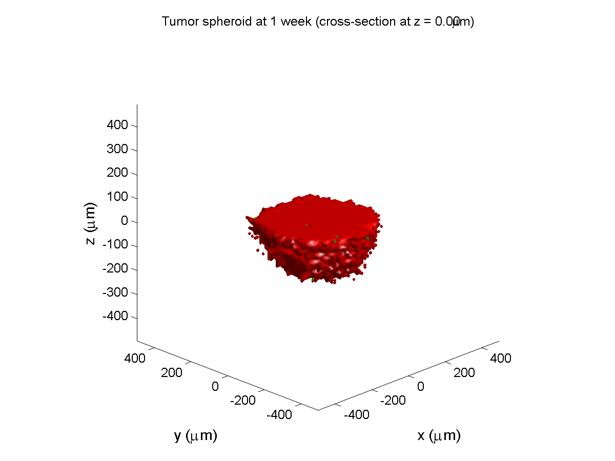
Oxygen- and space-limited growth are restricted to the outer boundary of the tumor spheroid.
2 weeks:
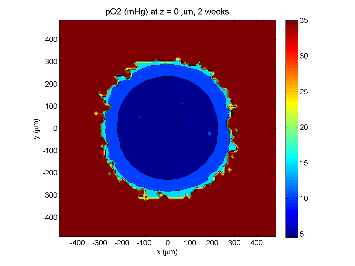
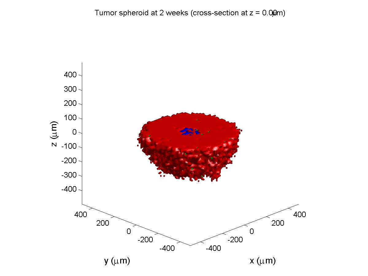
Oxygenation is dipped below 5 mmHg in the center, leading to necrosis.
3 weeks:
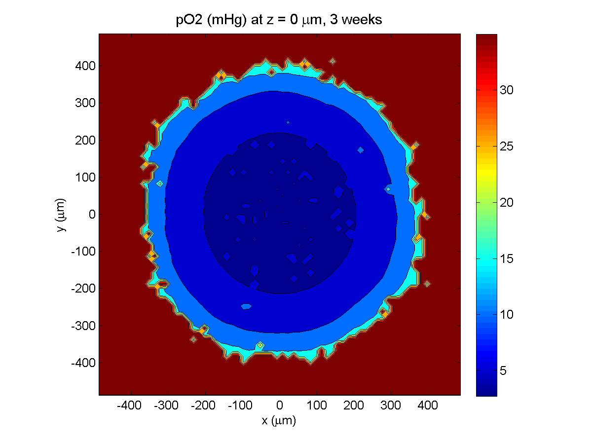
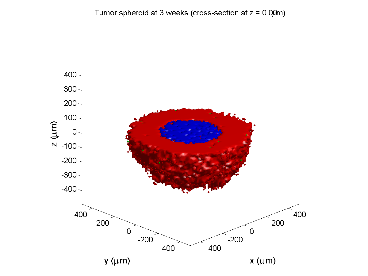
As the tumor grows, the hypoxic gradient increases, and the necrotic core grows. The code turns on a constant 5 micromolar dose of doxorubicin at this point
Treatment + 12 hours:
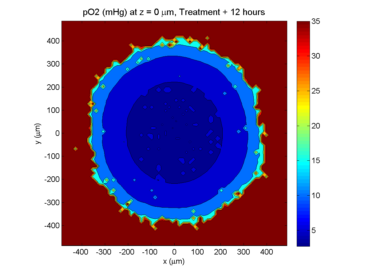
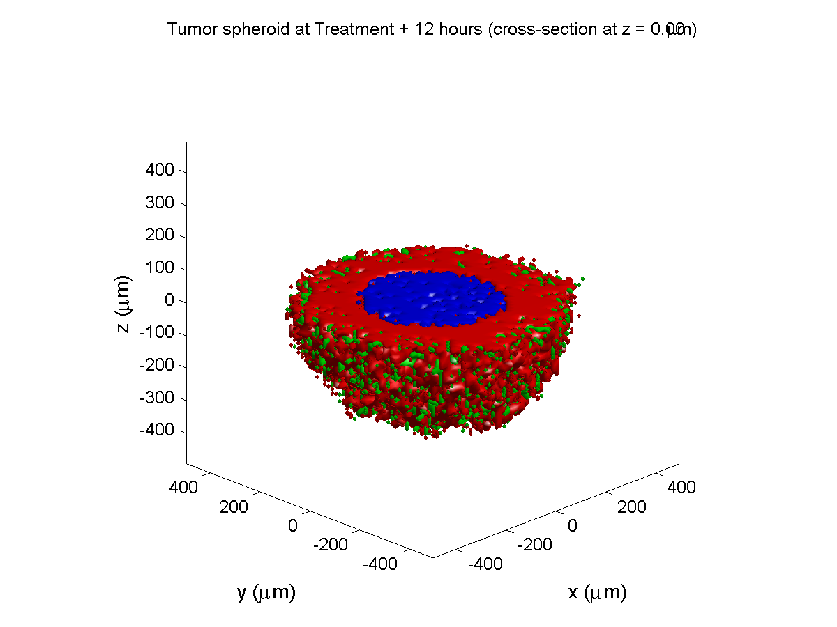

The drug has started to penetrate the tumor, triggering apoptotic death towards the outer periphery where exposure has been greatest.
Treatment + 24 hours:


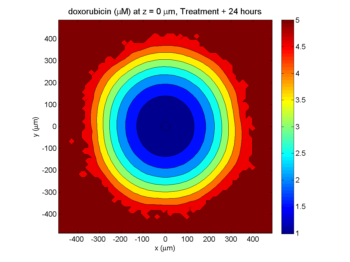
The drug profile hasn’t changed much, but the interior cells have now had greater exposure to drug, and hence greater response. Now apoptosis is observed throughout the non-necrotic tumor. The tumor has decreased in volume somewhat.
Treatment + 36 hours:
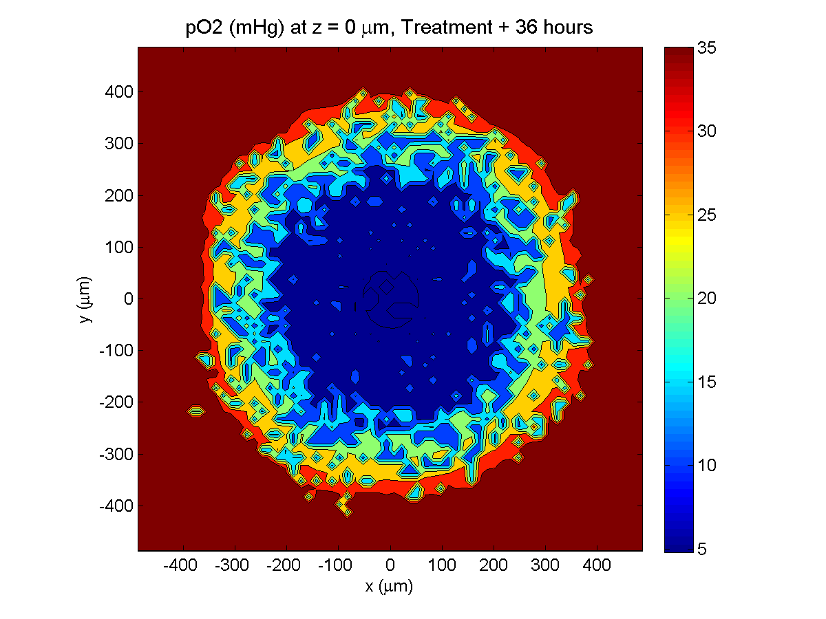
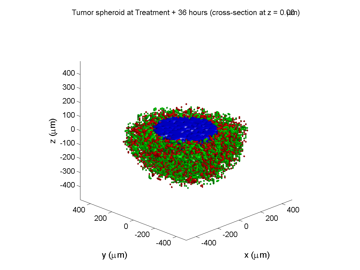
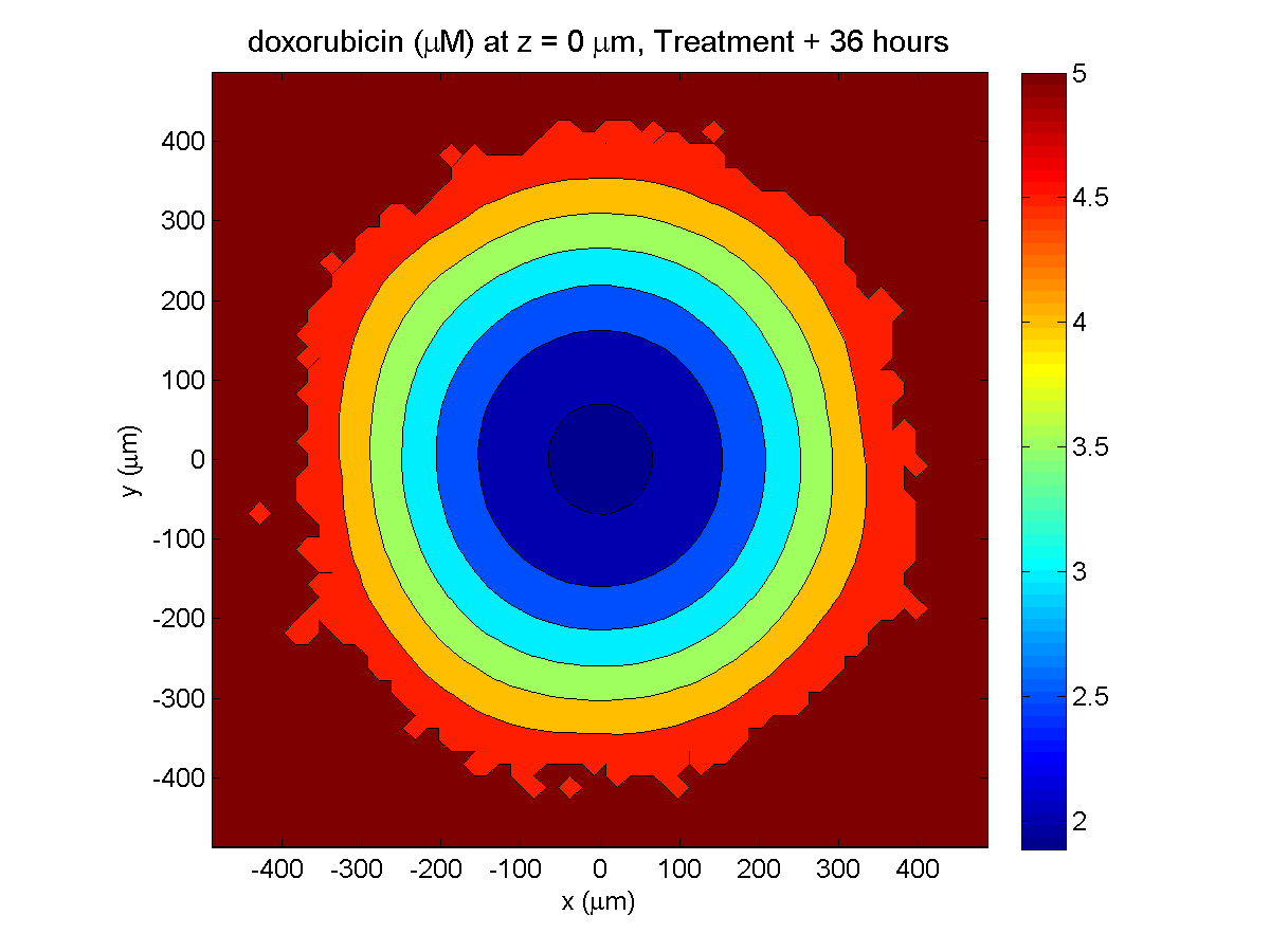
The non-necrotic tumor is now substantially apoptotic. We would require some pharamcokinetic effects (e.g., drug clearance, inactivation, or removal) to avoid the inevitable, presences of a pre-existing resistant strain, or emergence of resistance.
Treatment + 48 hours:
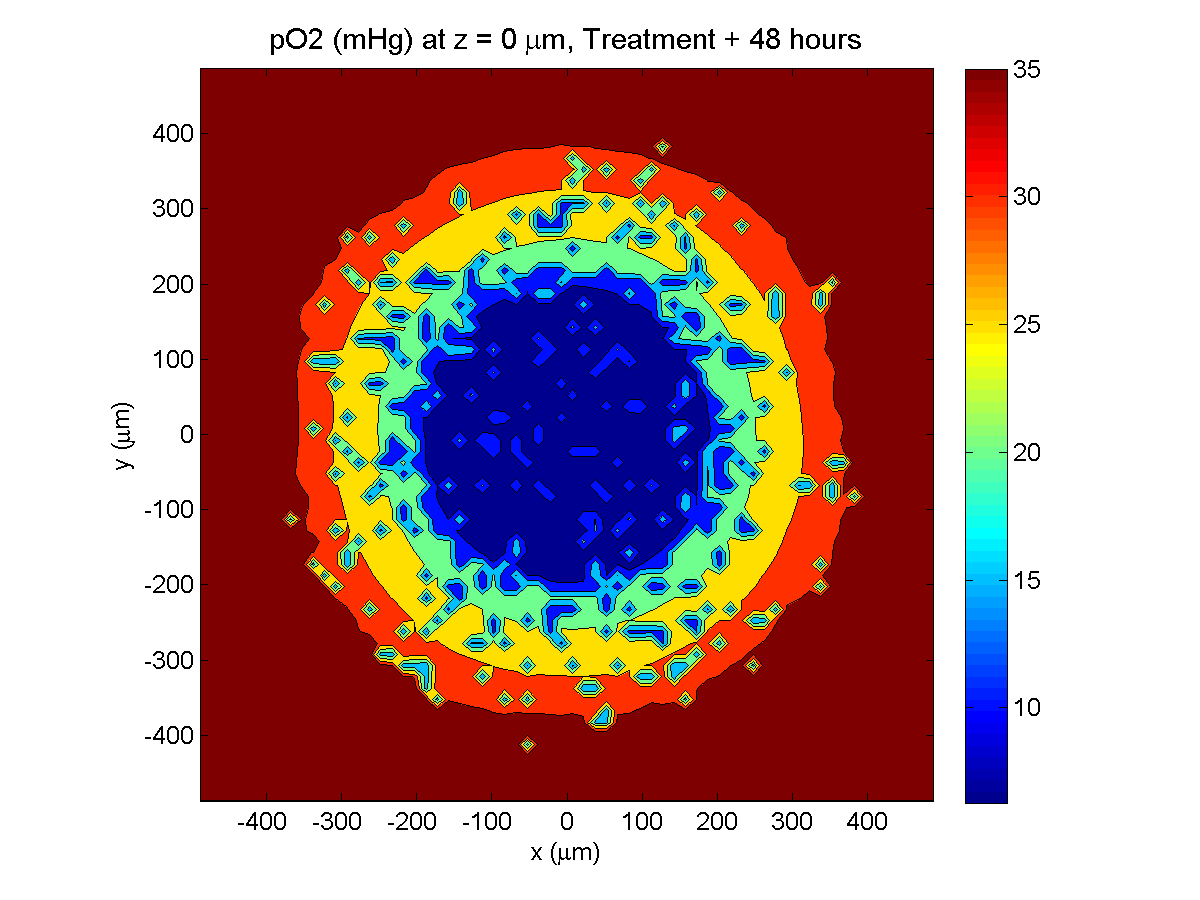
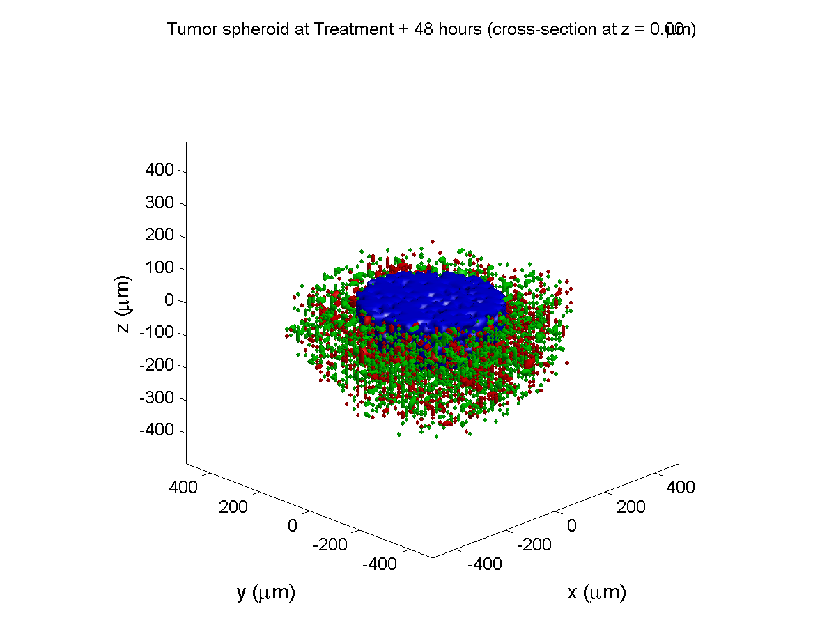
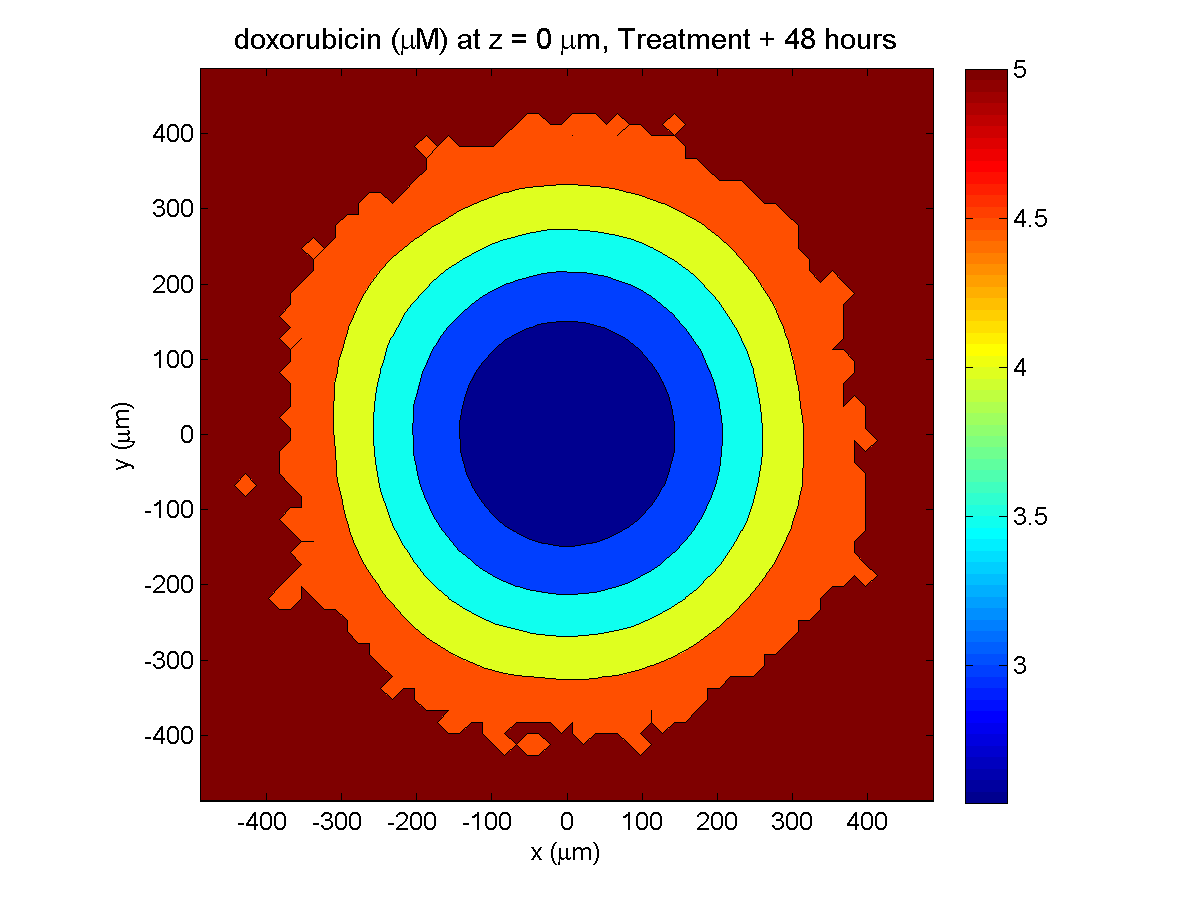
By now, almost all cells are apoptotic.
Treatment + 60 hours:

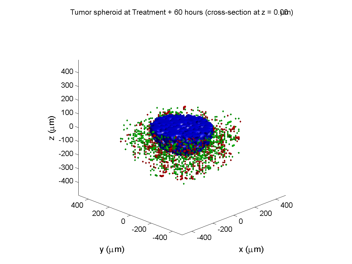

The non-necrotic tumor is nearly completed eliminated, leaving a leftover core of previously-necrotic cells (which did not change state in response to the drug–they were already dead!)
Source files
You can download completed source for this example here: https://sourceforge.net/projects/biofvm/files/Tutorials/Cellular_Automaton_1/
This file will include the following:
- BioFVM_cellular_automata.h
- BioFVM_cellular_automata.cpp
- BioFVM_CA_example_1.cpp
- read_MultiCellDS_xml.m (updated)
- plot_cellular_automata.m
- Makefile
What’s next
I plan to update this source code with extra cell motility, and potentially more realistic parameter values. Also, I plan to more formally separate out the example from the generic cell capabilities, so that this source code can work as a bona fide cellular automaton framework.
More immediately, my next tutorial will use the reverse strategy: start with an existing cellular automaton model, and integrate BioFVM capabilities.
Return to News • Return to MathCancer • Follow @MathCancer
Paul Macklin calls for common standards in cancer modeling
At a recent NCI-organized mini-symposium on big data in cancer, Paul Macklin called for new data standards in Multicellular data in simulations, experiments, and clinical science. USC featured the talk (abstract here) and the work at news.usc.edu.
Read the article: http://news.usc.edu/59091/usc-researcher-calls-for-common-standards-in-cancer-modeling/ (Feb. 21, 2014)
Macklin Lab featured on March 2013 cover of Notices of the American Mathematical Society
I’m very excited to be featured on this month’s cover of the Notices of the American Mathematical Society. The cover shows a series of images from a multiscale simulation of a tumor growing in the brain, made with John Lowengrub while I was a Ph.D. student at UC Irvine. (See Frieboes et al. 2007, Macklin et al. 2009, and Macklin and Lowengrub 2008.) The “about the cover” write-up (Page 325) gives more detail.
The inside has a short interview on our more current work, particularly 3-D agent-based modeling. You should also read Rick Durrett‘s perspective piece on cancer modeling (Page 304)—it’s a great read! (And yup, Figure 3 is from our patient-calibrated breast cancer modeling in Macklin et al. 2012. ;-) )
The entire March 2013 issue can be accessed for free at the AMS Notices website:
http://www.ams.org/notices/201303/
I want to thank Bill Casselman and Rick Durrett for making this possible. I had a lot of fun in the process, and I’m grateful for the opportunity to trade ideas!
DCIS modeling paper accepted
I am pleased to report that our paper has now been accepted. You can download the accepted preprint here. We also have a lot of supplementary material, including simulation movies, simulation datasets (for 0, 15, 30, adn 45 days of growth), and open source C++ code for postprocessing and visualization.
I discussed the results in detail here, but here’s the short version:
- We use a mechanistic, agent-based model of individual cancer cells growing in a duct. Cells are moved by adhesive and repulsive forces exchanged with other cells and the basement membrane. Cell phenotype is controlled by stochastic processes.
- We constrained all parameter expected to be relatively independent of patients by a careful analysis of the experimental biological and clinical literature.
- We developed the very first patient-specific calibration method, using clinically-accessible pathology. This is a key point in future patient-tailored predictions and surgical/therapeutic planning.
- The model made numerous quantitative predictions, such as:
- The tumor grows at a constant rate, between 7 to 10 mm/year. This is right in the middle of the range reported in the clinic.
- The tumor’s size in mammgraphy is linearly correlated with the post-surgical pathology size. When we linearly extrapolate our correlation across two orders of magnitude, it goes right through the middle of a cluster of 87 clinical data points.
- The tumor necrotic core has an age structuring: with oldest, calcified material in the center, and newest, most intact necrotic cells at the outer edge.
- The appearance of a “typical” DCIS duct cross-section varies with distance from the leading edge; all types of cross-sections predicted by our model are observed in patient pathology.
- The model also gave new insight on the underlying biology of breast cancer, such as:
- The split between the viable rim and necrotic core (observed almost universally in pathology) is not just an artifact, but an actual biomechanical effect from fast necrotic cell lysis.
- The constant rate of tumor growth arises from the biomechanical stress relief provided by lysing necrotic cells. This points to the critical role of intracellular and intra-tumoral water transport in determining the qualitative and quantitative behavior of tumors.
- Pyknosis (nuclear degradation in necrotic cells), must occur at a time scale between that of cell lysis (on the order of hours) and cell calcification (on the order of weeks).
- The current model cannot explain the full spectrum of calcification types; other biophysics, such as degradation over a long, 1-2 month time scale, must be at play.