Coarse-graining discrete cell cycle models
Introduction
One observation that often goes underappreciated in computational biology discussions is that a computational model is often a model of a model of a model of biology: that is, it’s a numerical approximation (a model) of a mathematical model of an experimental model of a real-life biological system. Thus, there are three big places where a computational investigation can fall flat:
- The experimental model may be a bad choice for the disease or process (not our fault).
- Second, the mathematical model of the experimental system may have flawed assumptions (something we have to evaluate).
- The numerical implementation may have bugs or otherwise be mathematically inconsistent with the mathematical model.
Critically, you can’t use simulations to evaluate the experimental model or the mathematical model until you verify that the numerical implementation is consistent with the mathematical model, and that the numerical solution converges as \( \Delta t\) and \( \Delta x \) shrink to zero.
There are numerous ways to accomplish this, but ideally, it boils down to having some analytical solutions to the mathematical model, and comparing numerical solutions to these analytical or theoretical results. In this post, we’re going to walk through the math of analyzing a typical type of discrete cell cycle model.
Discrete model
Suppose we have a cell cycle model consisting of phases \(P_1, P_2, \ldots P_n \), where cells in the \(P_i\) phase progress to the \(P_{i+1}\) phase after a mean waiting time of \(T_i\), and cells leaving the \(P_n\) phase divide into two cells in the \(P_1\) phase. Assign each cell agent \(k\) a current phenotypic phase \( S_k(t) \). Suppose also that each phase \( i \) has a death rate \( d_i \), and that cells persist for on average \( T_\mathrm{A} \) time in the dead state before they are removed from the simulation.
The mean waiting times \( T_i \) are equivalent to transition rates \( r_i = 1 / T_i \) (Macklin et al. 2012). Moreover, for any time interval \( [t,t+\Delta t] \), both are equivalent to a transition probability of
\[ \mathrm{Prob}\Bigl( S_k(t+\Delta t) = P_{i+1} | S(t) = P_i \Bigr) = 1 – e^{ -r_i \Delta t } \approx r_i \Delta t = \frac{ \Delta t}{ T_i}. \] In many discrete models (especially cellular automaton models) with fixed step sizes \( \Delta t \), models are stated in terms of transition probabilities \( p_{i,i+1} \), which we see are equivalent to the work above with \( p_{i,i+1} = r_i \Delta t = \Delta t / T_i \), allowing us to tie mathematical model forms to biological, measurable parameters. We note that each \(T_i\) is the average duration of the \( P_i \) phase.
Concrete example: a Ki67 Model
Ki-67 is a nuclear protein that is expressed through much of the cell cycle, including S, G2, M, and part of G1 after division. It is used very commonly in pathology to assess proliferation, particularly in cancer. See the references and discussion in (Macklin et al. 2012). In Macklin et al. (2012), we came up with a discrete cell cycle model to match Ki-67 data (along with cleaved Caspase-3 stains for apoptotic cells). Let’s summarize the key parts here.
Each cell agent \(i\) has a phase \(S_i(t)\). Ki67- cells are quiescent (phase \(Q\), mean duration \( T_\mathrm{Q} \)), and they can enter the Ki67+ \(K_1\) phase (mean duration \(T_1\)). When \( K_1 \) cells leave their phase, they divide into two Ki67+ daughter cells in the \( K_2 \) phase with mean duration \( T_2 \). When cells exit \( K_2 \), they return to \( Q \). Cells in any phase can become apoptotic (enter the \( A \) phase with mean duration \( T_\mathrm{A} \)), with death rate \( r_\mathrm{A} \).
Coarse-graining to an ODE model
If each phase \(i\) has a death rate \(d_i\), if \( N_i(t) \) denotes the number of cells in the \( P_i \) phase at time \( t\), and if \( A(t) \) is the number of dead (apoptotic) cells at time \( t\), then on average, the number of cells in the \( P_i \) phase at the next time step is given by
\[ N_i(t+\Delta t) = N_i(t) + N_{i-1}(t) \cdot \left[ \textrm{prob. of } P_{i-1} \rightarrow P_i \textrm{ transition} \right] – N_i(t) \cdot \left[ \textrm{prob. of } P_{i} \rightarrow P_{i+1} \textrm{ transition} \right] \] \[ – N_i(t) \cdot \left[ \textrm{probability of death} \right] \] By the work above, this is:
\[ N_i(t+\Delta t) \approx N_i(t) + N_{i-1}(t) r_{i-1} \Delta t – N_i(t) r_i \Delta t – N_i(t) d_i \Delta t , \] or after shuffling terms and taking the limit as \( \Delta t \downarrow 0\), \[ \frac{d}{dt} N_i(t) = r_{i-1} N_{i-1}(t) – \left( r_i + d_i \right) N_i(t). \] Continuing this analysis, we obtain a linear system:
\[ \frac{d}{dt}{ \vec{N} } = \begin{bmatrix} -(r_1+d_1) & 0 & \cdots & 0 & 2r_n & 0 \\ r_1 & -(r_2+d_2) & 0 & \cdots & 0 & 0 \\ 0 & r_2 & -(r_3+d_3) & 0 & \cdots & 0 \\ & & \ddots & & \\0&\cdots&0 &r_{n-1} & -(r_n+d_n) & 0 \\ d_1 & d_2 & \cdots & d_{n-1} & d_n & -\frac{1}{T_\mathrm{A}} \end{bmatrix}\vec{N} = M \vec{N}, \] where \( \vec{N}(t) = [ N_1(t), N_2(t) , \ldots , N_n(t) , A(t) ] \).
For the Ki67 model above, let \(\vec{N} = [K_1, K_2, Q, A]\). Then the linear system is
\[ \frac{d}{dt} \vec{N} = \begin{bmatrix} -\left( \frac{1}{T_1} + r_\mathrm{A} \right) & 0 & \frac{1}{T_\mathrm{Q}} & 0 \\ \frac{2}{T_1} & -\left( \frac{1}{T_2} + r_\mathrm{A} \right) & 0 & 0 \\ 0 & \frac{1}{T_2} & -\left( \frac{1}{T_\mathrm{Q}} + r_\mathrm{A} \right) & 0 \\ r_\mathrm{A} & r_\mathrm{A} & r_\mathrm{A} & -\frac{1}{T_\mathrm{A}} \end{bmatrix} \vec{N} .\]
(If we had written \( \vec{N} = [Q, K_1, K_2 , A] \), then the matrix above would have matched the general form.)
Some theoretical results
If \( M\) has eigenvalues \( \lambda_1 , \ldots \lambda_{n+1} \) and corresponding eigenvectors \( \vec{v}_1, \ldots , \vec{v}_{n+1} \), then the general solution is given by
\[ \vec{N}(t) = \sum_{i=1}^{n+1} c_i e^{ \lambda_i t } \vec{v}_i ,\] and if the initial cell counts are given by \( \vec{N}(0) \) and we write \( \vec{c} = [c_1, \ldots c_{n+1} ] \), we can obtain the coefficients by solving \[ \vec{N}(0) = [ \vec{v}_1 | \cdots | \vec{v}_{n+1} ]\vec{c} .\] In many cases, it turns out that all but one of the eigenvalues (say \( \lambda \) with corresponding eigenvector \(\vec{v}\)) are negative. In this case, all the other components of the solution decay away, and for long times, we have \[ \vec{N}(t) \approx c e^{ \lambda t } \vec{v} .\] This is incredibly useful, because it says that over long times, the fraction of cells in the \( i^\textrm{th} \) phase is given by \[ v_{i} / \sum_{j=1}^{n+1} v_{j}. \]
Matlab implementation (with the Ki67 model)
First, let’s set some parameters, to make this a little easier and reusable.
parameters.dt = 0.1; % 6 min = 0.1 hours
parameters.time_units = 'hour';
parameters.t_max = 3*24; % 3 days

parameters.K1.duration =  13;
parameters.K1.death_rate = 1.05e-3;
parameters.K1.initial = 0;

parameters.K2.duration = 2.5;
parameters.K2.death_rate = 1.05e-3;
parameters.K2.initial = 0;

parameters.Q.duration = 74.35 ;
parameters.Q.death_rate = 1.05e-3;
parameters.Q.initial = 1000;

parameters.A.duration = 8.6;
parameters.A.initial = 0;
Next, we write a function to read in the parameter values, construct the matrix (and all the data structures), find eigenvalues and eigenvectors, and create the theoretical solution. It also finds the positive eigenvalue to determine the long-time values.
function solution = Ki67_exact( parameters )

% allocate memory for the main outputs

solution.T = 0:parameters.dt:parameters.t_max;
solution.K1 = zeros( 1 , length(solution.T));
solution.K2 = zeros( 1 , length(solution.T));
solution.K = zeros( 1 , length(solution.T));
solution.Q = zeros( 1 , length(solution.T));
solution.A = zeros( 1 , length(solution.T));
solution.Live = zeros( 1 , length(solution.T));
solution.Total = zeros( 1 , length(solution.T));

% allocate memory for cell fractions

solution.AI = zeros(1,length(solution.T));
solution.KI1 = zeros(1,length(solution.T));
solution.KI2 = zeros(1,length(solution.T));
solution.KI = zeros(1,length(solution.T));

% get the main parameters

T1 = parameters.K1.duration;
r1A = parameters.K1.death_rate;

T2 = parameters.K2.duration;
r2A = parameters.K2.death_rate;

TQ = parameters.Q.duration;
rQA = parameters.Q.death_rate;

TA = parameters.A.duration;

% write out the mathematical model:
% d[Populations]/dt = Operator*[Populations]

Operator = [ -(1/T1 +r1A) , 0 , 1/TQ , 0; ...
    2/T1 , -(1/T2 + r2A) ,0 , 0; ...
    0 , 1/T2 , -(1/TQ + rQA) , 0; ...
    r1A , r2A, rQA , -1/TA ];

% eigenvectors and eigenvalues

[V,D] = eig(Operator);
eigenvalues = diag(D);

% save the eigenvectors and eigenvalues in case you want them.

solution.V = V;
solution.D = D;
solution.eigenvalues = eigenvalues;

% initial condition

VecNow = [ parameters.K1.initial ; parameters.K2.initial ; ...
    parameters.Q.initial ; parameters.A.initial ] ;
solution.K1(1) = VecNow(1);
solution.K2(1) = VecNow(2);
solution.Q(1) = VecNow(3);
solution.A(1) = VecNow(4);
solution.K(1) = solution.K1(1) + solution.K2(1);
solution.Live(1) = sum( VecNow(1:3) );
solution.Total(1) = sum( VecNow(1:4) );

solution.AI(1) = solution.A(1) / solution.Total(1);
solution.KI1(1) = solution.K1(1) / solution.Total(1);
solution.KI2(1) = solution.K2(1) / solution.Total(1);
solution.KI(1) = solution.KI1(1) + solution.KI2(1);

% now, get the coefficients to write the analytic solution
% [Populations] = c1*V(:,1)*exp( d(1,1)*t) + c2*V(:,2)*exp( d(2,2)*t ) +
%                 c3*V(:,3)*exp( d(3,3)*t) + c4*V(:,4)*exp( d(4,4)*t );

coeff = linsolve( V , VecNow );

% find the (hopefully one) positive eigenvalue.
% eigensolutions with negative eigenvalues decay,
% leaving this as the long-time behavior.

eigenvalues = diag(D);
n = find( real( eigenvalues ) > 0 )
solution.long_time.KI1 = V(1,n) / sum( V(:,n) );
solution.long_time.KI2 = V(2,n) / sum( V(:,n) );
solution.long_time.QI = V(3,n) / sum( V(:,n) );
solution.long_time.AI = V(4,n) / sum( V(:,n) ) ;
solution.long_time.KI = solution.long_time.KI1 + solution.long_time.KI2;

% now, write out the solution at all the times
for i=2:length( solution.T )
    % compact way to write the solution
    VecExact = real( V*( coeff .* exp( eigenvalues*solution.T(i) ) ) );

    solution.K1(i) = VecExact(1);
    solution.K2(i) = VecExact(2);
    solution.Q(i) = VecExact(3);
    solution.A(i) = VecExact(4);
    solution.K(i) = solution.K1(i) + solution.K2(i);
    solution.Live(i) = sum( VecExact(1:3) );
    solution.Total(i) = sum( VecExact(1:4) );

    solution.AI(i) = solution.A(i) / solution.Total(i);
    solution.KI1(i) = solution.K1(i) / solution.Total(i);
    solution.KI2(i) = solution.K2(i) / solution.Total(i);
    solution.KI(i) = solution.KI1(i) + solution.KI2(i);
end

return;
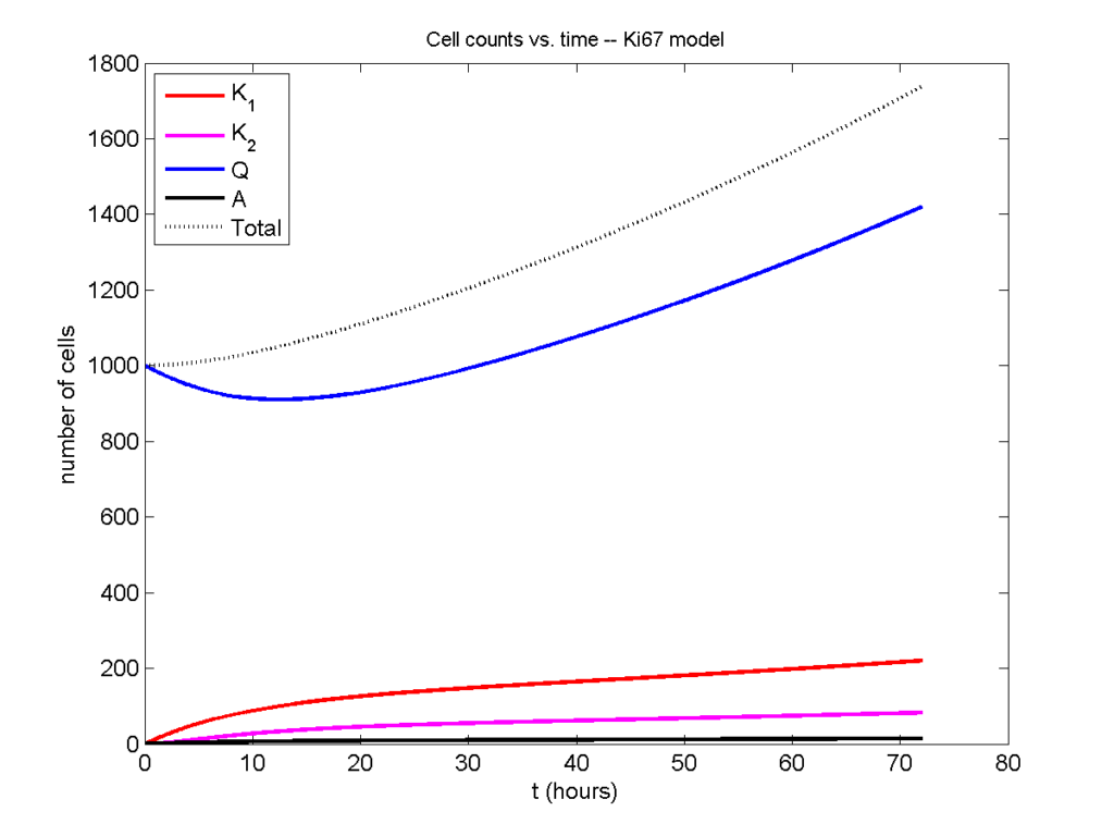
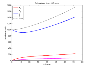
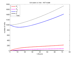
Now, let’s run it and see what this thing looks like:
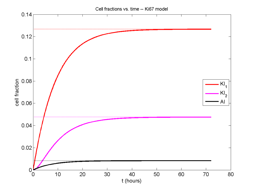
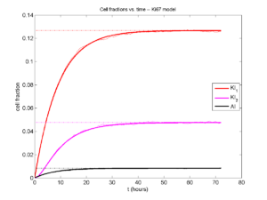
Next, we plot KI1, KI2, and AI versus time (solid curves), along with the theoretical long-time behavior (dashed curves). Notice how well it matches–it’s neat when theory works! :-)
Some readers may recognize the long-time fractions: KI1 + KI2 = KI = 0.1743, and AI = 0.00833, very close to the DCIS patient values from our simulation study in Macklin et al. (2012) and improved calibration work in Hyun and Macklin (2013).
Comparing simulations and theory
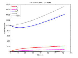
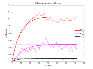
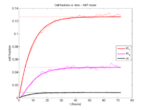
I wrote a small Matlab program to implement the discrete model: start with 1000 cells in the \(Q\) phase, and in each time interval \([t,t+\Delta t]\), each cell “decides” whether to advance to the next phase, stay in the same phase, or apoptose. If we compare a single run against the theoretical curves, we see hints of a match:
If we average 10 simulations and compare, the match is better:
And lastly, if we average 100 simulations and compare, the curves are very difficult to tell apart:
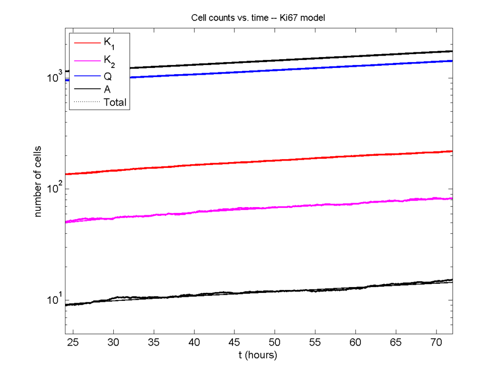
Even in logarithmic space, it’s tough to tell these apart:
Code
The following matlab files (available here) can be used to reproduce this post:
- Ki67_exact.m
- The function defined above to create the exact solution using the eigenvalue/eignvector approach.
- Ki67_stochastic.m
- Runs a single stochastic simulation, using the supplied parameters.
- script.m
- Runs the theoretical solution first, creates plots, and then runs the stochastic model 100 times for comparison.
To make it all work, simply run “script” at the command prompt. Please note that it will generate some png files in its directory.
Closing thoughts
In this post, we showed a nice way to check a discrete model against theoretical behavior–both in short-term dynamics and long-time behavior. The same work should apply to validating many discrete models. However, when you add spatial effects (e.g., a cellular automaton model that won’t proliferate without an empty neighbor site), I wouldn’t expect a match. (But simulating cells that initially have a “salt and pepper”, random distribution should match this for early times.)
Moreover, models with deterministic phase durations (e.g., K1, K2, and A have fixed durations) aren’t consistent with the ODE model above, unless the cells they are each initialized with a random amount of “progress” in their initial phases. (Otherwise, the cells in each phase will run synchronized, and there will be fixed delays before cells transition to other phases.) Delay differential equations better describe such models. However, for long simulation times, the slopes of the sub-populations and the cell fractions should start to better and better match the ODE models.
Now that we have verified that the discrete model is performing as expected, we can have greater confidence in its predictions, and start using those predictions to assess the underlying models. In ODE and PDE models, you often validate the code on simpler problems where you have an analytical solution, and then move on to making simulation predictions in cases where you can’t solve analytically. Similarly, we can now move on to variants of the discrete model where we can’t as easily match ODE theory (e.g., time-varying rate parameters, spatial effects), but with the confidence that the phase transitions are working as they should.
