Category: modeling
User parameters in PhysiCell
As of release 1.4.0, users can add any number of Boolean, integer, double, and string parameters to an XML configuration file. (These are stored by default in ./config/. The default parameter file is ./config/PhysiCell_settings.xml.) These parameters are automatically parsed into a parameters data structure, and accessible throughout a PhysiCell project.
This tutorial will show you the key techniques to use these features. (See the User_Guide for full documentation.) First, let’s create a barebones 2D project by populating the 2D template project. In a terminal shell in your root PhysiCell directory, do this:
make template2D
We will use this 2D project template for the remainder of the tutorial. We assume you already have a working copy of PhysiCell installed, version 1.4.0 or later. (If not, visit the PhysiCell tutorials to find installation instructions for your operating system.)
User parameters in the XML configuration file
Next, let’s look at the parameter file. In your text editor of choice, open up ./config/PhysiCell_settings.xml, and browse down to <user_parameters>, which will have some sample parameters from the 2D template project.
	<user_parameters>
		<random_seed type="int" units="dimensionless">0</random_seed>
		<!-- example parameters from the template -->

		<!-- motile cell type parameters -->
		<motile_cell_persistence_time type="double" units="min">15</motile_cell_persistence_time>
		<motile_cell_migration_speed type="double" units="micron/min">0.5</motile_cell_migration_speed>
		<motile_cell_relative_adhesion type="double" units="dimensionless">0.05</motile_cell_relative_adhesion>
		<motile_cell_apoptosis_rate type="double" units="1/min">0.0</motile_cell_apoptosis_rate>
		<motile_cell_relative_cycle_entry_rate type="double" units="dimensionless">0.1</motile_cell_relative_cycle_entry_rate>
	</user_parameters>
Notice a few trends:
- Each XML element (tag) under <user_parameters> is a user parameter, whose name is the element name.
- Each variable requires an attribute named “type”, with one of the following four values:
- bool for a Boolean parameter
- int for an integer parameter
- double for a double (floating point) parameter
- string for text string parameter
While we do not encourage it, if no valid type is supplied, PhysiCell will attempt to interpret the parameter as a double.
- Each variable here has an (optional) attribute “units”. PhysiCell does not convert units, but these are helpful for clarity between users and developers. By default, PhysiCell uses minutes for all time units, and microns for all spatial units.
- Then, between the tags, you list the value of your parameter.
Let’s add the following parameters to the configuration file:
- A string parameter called motile_color that sets the color of the motile_cell type in SVG outputs. Please refer to the User Guide (in the documentation folder) for more information on allowed color formats, including rgb values and named colors. Let’s use the value darkorange.
- A double parameter called base_cycle_entry_rate that will give the rate of entry to the S cycle phase from the G1 phase for the default cell type in the code. Let’s use a ridiculously high value of 0.01 min-1.
- A double parameter called base_apoptosis_rate for the default cell type. Let’s set the value at 1e-7 min-1.
- A double parameter that sets the (relative) maximum cell-cell adhesion sensing distance, relative to the cell’s radius. Let’s set it at 2.5 (dimensionless). (The default is 1.25.)
- A bool parameter that enables or disables placing a single motile cell in the initial setup. Let’s set it at true.
If you edit the <user_parameters> to include these, it should look like this:
	<user_parameters>
		<random_seed type="int" units="dimensionless">0</random_seed>
		<!-- example parameters from the template -->

		<!-- motile cell type parameters -->
		<motile_cell_persistence_time type="double" units="min">15</motile_cell_persistence_time>
		<motile_cell_migration_speed type="double" units="micron/min">0.5</motile_cell_migration_speed>
		<motile_cell_relative_adhesion type="double" units="dimensionless">0.05</motile_cell_relative_adhesion>
		<motile_cell_apoptosis_rate type="double" units="1/min">0.0</motile_cell_apoptosis_rate>
		<motile_cell_relative_cycle_entry_rate type="double" units="dimensionless">0.1</motile_cell_relative_cycle_entry_rate>

		<!-- for the tutorial -->
		<motile_color type="string" units="dimensionless">darkorange</motile_color>

		<base_cycle_entry_rate type="double" units="1/min">0.01</base_cycle_entry_rate>
		<base_apoptosis_rate type="double" units="1/min">1e-7</base_apoptosis_rate>
		<base_cell_adhesion_distance type="double" units="dimensionless">2.5</base_cell_adhesion_distance>

		<include_motile_cell type="bool" units="dimensionless">true</include_motile_cell>
	</user_parameters>
Viewing the loaded parameters
Let’s compile and run the project.
make
./project2D
At the beginning of the simulation, PhysiCell parses the <user_parameters> block into a global data structure called parameters, with sub-parts bools, ints, doubles, and strings. It displays these loaded parameters at the start of the simulation. Here’s what it looks like:
shell$  ./project2D
Using config file ./config/PhysiCell_settings.xml ...
User parameters in XML config file:
Bool parameters::
include_motile_cell: 1 [dimensionless]

Int parameters::
random_seed: 0 [dimensionless]

Double parameters::
motile_cell_persistence_time: 15 [min]
motile_cell_migration_speed: 0.5 [micron/min]
motile_cell_relative_adhesion: 0.05 [dimensionless]
motile_cell_apoptosis_rate: 0 [1/min]
motile_cell_relative_cycle_entry_rate: 0.1 [dimensionless]
base_cycle_entry_rate: 0.01 [1/min]
base_apoptosis_rate: 1e-007 [1/min]
base_cell_adhesion_distance: 2.5 [dimensionless]

String parameters::
motile_color: darkorange [dimensionless]
Getting parameter values
Within a PhysiCell project, you can access the value of any parameter by either its index or its name, so long as you know its type. Here’s an example of accessing the base_cell_adhesion_distance by its name:
/* this directly accesses the value of the parameter */
double temp = parameters.doubles( "base_cell_adhesion_distance" );
std::cout << temp << std::endl;

/* this streams a formatted output including the parameter name and units */
std::cout << parameters.doubles[ "base_cell_adhesion_distance" ] << std::endl;

std::cout << parameters.doubles["base_cell_adhesion_distance"].name << " "
     << parameters.doubles["base_cell_adhesion_distance"].value << " "
     << parameters.doubles["base_cell_adhesion_distance"].units << std::endl;
Notice that accessing by () gets the value of the parameter in a user-friendly way, whereas accessing by [] gets the entire parameter, including its name, value, and units.
You can more efficiently access the parameter by first finding its integer index, and accessing by index:
/* this directly accesses the value of the parameter */
int my_index = parameters.doubles.find_index( "base_cell_adhesion_distance" );
double temp = parameters.doubles( my_index );
std::cout << temp << std::endl;

/* this streams a formatted output including the parameter name and units */
std::cout << parameters.doubles[ my_index ] << std::endl;

std::cout << parameters.doubles[ my_index ].name << " "
     << parameters.doubles[ my_index ].value << " "
     << parameters.doubles[ my_index ].units << std::endl;
Similarly, we can access string and Boolean parameters. For example:
if( parameters.bools("include_motile_cell") == true )
{ std::cout << "I shall include a motile cell." << std::endl; }

int rand_ind = parameters.ints.find_index( "random_seed" );
std::cout << parameters.ints[rand_ind].name << " is at index " << rand_ind << std::endl;

std::cout << "We'll use this nice color: " << parameters.strings( "motile_color" );
Using the parameters in custom functions
Let’s use these new parameters when setting up the parameter values of the simulation. For this project, all custom code is in ./custom_modules/custom.cpp. Open that source file in your favorite text editor. Look for the function called “create_cell_types“. In the code snipped below, we access the parameter values to set the appropriate parameters in the default cell definition, rather than hard-coding them.
	// add custom data here, if any

	/* for the tutorial */
	cell_defaults.phenotype.cycle.data.transition_rate(G0G1_index,S_index) =
		parameters.doubles("base_cycle_entry_rate");
	cell_defaults.phenotype.death.rates[apoptosis_model_index] =
		parameters.doubles("base_apoptosis_rate");

	cell_defaults.phenotype.mechanics.set_relative_maximum_adhesion_distance(
		parameters.doubles("base_cell_adhesion_distance") );
Next, let’s change the tissue setup (“setup_tissue“) to check our Boolean variable before placing the initial motile cell.
     // now create a motile cell
     /*  remove this conditional for the normal project */
     if( parameters.bools("include_motile_cell") == true )
     {
           pC = create_cell( motile_cell );
           pC->assign_position( 15.0, -18.0, 0.0 );
     }
Lastly, let’s make use of the string parameter to change the plotting. Search for my_coloring_function and edit the source file to use the new color:
	// if the cell is motile and not dead, paint it black

	static std::string motile_color = parameters.strings( "motile_color" );  // tutorial

	if( pCell->phenotype.death.dead == false && pCell->type == 1 )
	{
		 output[0] = motile_color;
		 output[2] = motile_color;
	}
Notice the static here: We intend to call this function many, many times. For performance reasons, we don’t want to declare a string, instantiate it with motile_color, pass it to parameters.strings(), and then deallocate it once done. Instead, we store the search statically within the function, so that all future function calls will have access to that search result.
And that’s it! Compile your code, and give it a go.
make
./project2D
This should create a lot of data in the ./output directory, including SVG files that color motile cells as darkorange, like this one below.
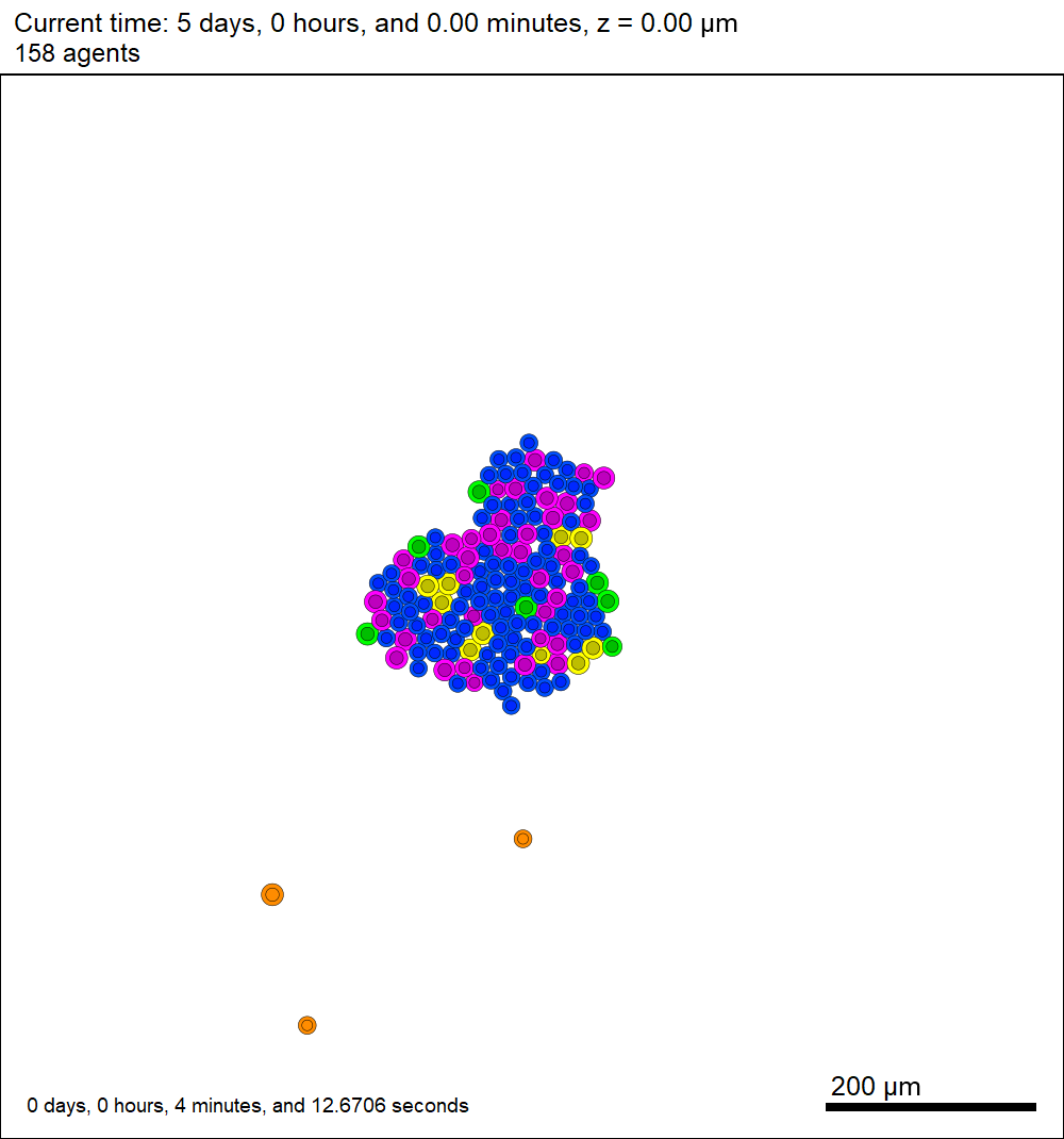
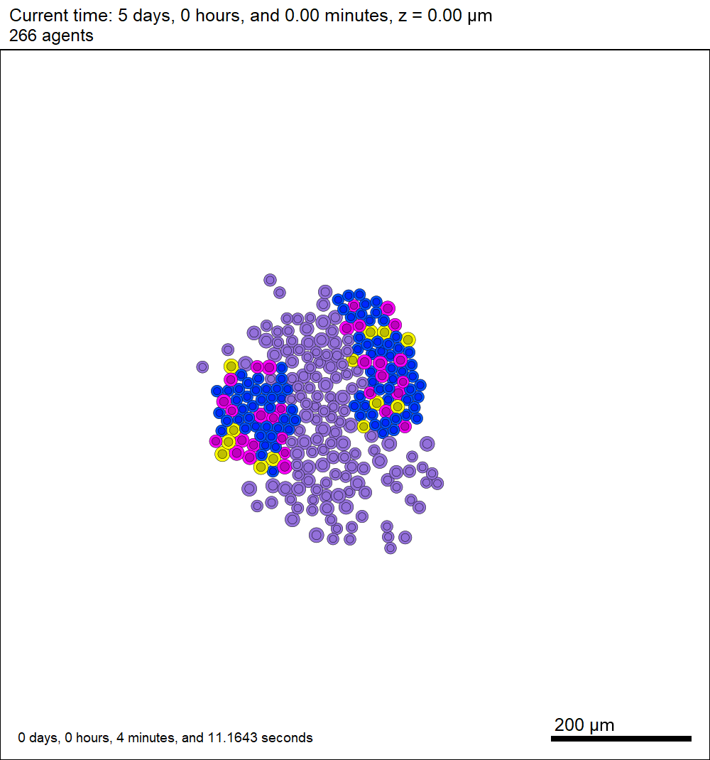
Now that this project is parsing the XML file to get parameter values, we don’t need to recompile to change a model parameter. For example, change motile_color to mediumpurple, set motile_cell_migration_speed to 0.25, and set motile_cell_relative_cycle_entry_rate to 2.0. Rerun the code (without compiling):
./project2D
And let’s look at the change in the final SVG output (output00000120.svg):
More notes on configuration files
You may notice other sections in the XML configuration file. I encourage you to explore them, but the meanings should be evident: you can set the computational domain size, the number of threads (for OpenMP parallelization), and how frequently (and where) data are stored. In future PhysiCell releases, we will continue adding more and more options to these XML files to simplify setup and configuration of PhysiCell models.
Coarse-graining discrete cell cycle models
Introduction
One observation that often goes underappreciated in computational biology discussions is that a computational model is often a model of a model of a model of biology: that is, it’s a numerical approximation (a model) of a mathematical model of an experimental model of a real-life biological system. Thus, there are three big places where a computational investigation can fall flat:
- The experimental model may be a bad choice for the disease or process (not our fault).
- Second, the mathematical model of the experimental system may have flawed assumptions (something we have to evaluate).
- The numerical implementation may have bugs or otherwise be mathematically inconsistent with the mathematical model.
Critically, you can’t use simulations to evaluate the experimental model or the mathematical model until you verify that the numerical implementation is consistent with the mathematical model, and that the numerical solution converges as \( \Delta t\) and \( \Delta x \) shrink to zero.
There are numerous ways to accomplish this, but ideally, it boils down to having some analytical solutions to the mathematical model, and comparing numerical solutions to these analytical or theoretical results. In this post, we’re going to walk through the math of analyzing a typical type of discrete cell cycle model.
Discrete model
Suppose we have a cell cycle model consisting of phases \(P_1, P_2, \ldots P_n \), where cells in the \(P_i\) phase progress to the \(P_{i+1}\) phase after a mean waiting time of \(T_i\), and cells leaving the \(P_n\) phase divide into two cells in the \(P_1\) phase. Assign each cell agent \(k\) a current phenotypic phase \( S_k(t) \). Suppose also that each phase \( i \) has a death rate \( d_i \), and that cells persist for on average \( T_\mathrm{A} \) time in the dead state before they are removed from the simulation.
The mean waiting times \( T_i \) are equivalent to transition rates \( r_i = 1 / T_i \) (Macklin et al. 2012). Moreover, for any time interval \( [t,t+\Delta t] \), both are equivalent to a transition probability of
\[ \mathrm{Prob}\Bigl( S_k(t+\Delta t) = P_{i+1} | S(t) = P_i \Bigr) = 1 – e^{ -r_i \Delta t } \approx r_i \Delta t = \frac{ \Delta t}{ T_i}. \] In many discrete models (especially cellular automaton models) with fixed step sizes \( \Delta t \), models are stated in terms of transition probabilities \( p_{i,i+1} \), which we see are equivalent to the work above with \( p_{i,i+1} = r_i \Delta t = \Delta t / T_i \), allowing us to tie mathematical model forms to biological, measurable parameters. We note that each \(T_i\) is the average duration of the \( P_i \) phase.
Concrete example: a Ki67 Model
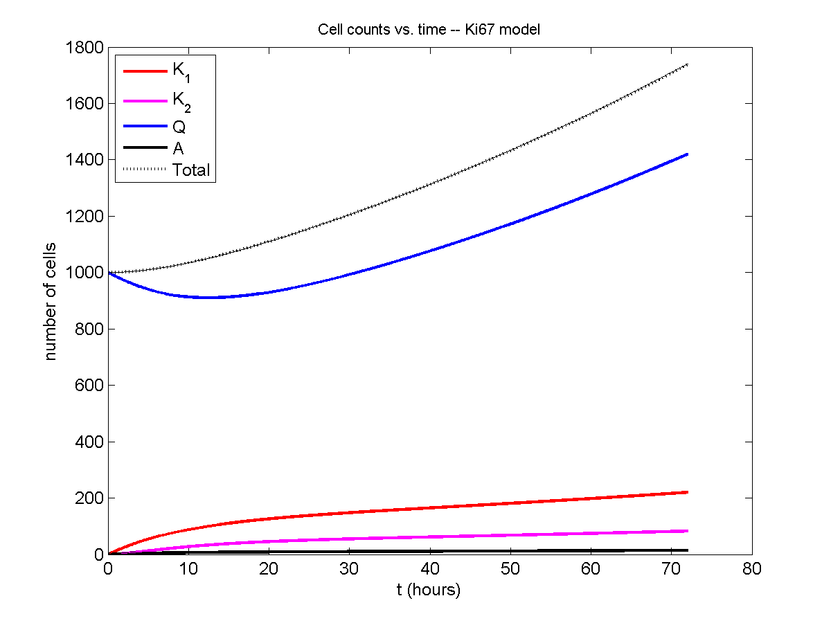
Ki-67 is a nuclear protein that is expressed through much of the cell cycle, including S, G2, M, and part of G1 after division. It is used very commonly in pathology to assess proliferation, particularly in cancer. See the references and discussion in (Macklin et al. 2012). In Macklin et al. (2012), we came up with a discrete cell cycle model to match Ki-67 data (along with cleaved Caspase-3 stains for apoptotic cells). Let’s summarize the key parts here.
Each cell agent \(i\) has a phase \(S_i(t)\). Ki67- cells are quiescent (phase \(Q\), mean duration \( T_\mathrm{Q} \)), and they can enter the Ki67+ \(K_1\) phase (mean duration \(T_1\)). When \( K_1 \) cells leave their phase, they divide into two Ki67+ daughter cells in the \( K_2 \) phase with mean duration \( T_2 \). When cells exit \( K_2 \), they return to \( Q \). Cells in any phase can become apoptotic (enter the \( A \) phase with mean duration \( T_\mathrm{A} \)), with death rate \( r_\mathrm{A} \).
Coarse-graining to an ODE model
If each phase \(i\) has a death rate \(d_i\), if \( N_i(t) \) denotes the number of cells in the \( P_i \) phase at time \( t\), and if \( A(t) \) is the number of dead (apoptotic) cells at time \( t\), then on average, the number of cells in the \( P_i \) phase at the next time step is given by
\[ N_i(t+\Delta t) = N_i(t) + N_{i-1}(t) \cdot \left[ \textrm{prob. of } P_{i-1} \rightarrow P_i \textrm{ transition} \right] – N_i(t) \cdot \left[ \textrm{prob. of } P_{i} \rightarrow P_{i+1} \textrm{ transition} \right] \] \[ – N_i(t) \cdot \left[ \textrm{probability of death} \right] \] By the work above, this is:
\[ N_i(t+\Delta t) \approx N_i(t) + N_{i-1}(t) r_{i-1} \Delta t – N_i(t) r_i \Delta t – N_i(t) d_i \Delta t , \] or after shuffling terms and taking the limit as \( \Delta t \downarrow 0\), \[ \frac{d}{dt} N_i(t) = r_{i-1} N_{i-1}(t) – \left( r_i + d_i \right) N_i(t). \] Continuing this analysis, we obtain a linear system:
\[ \frac{d}{dt}{ \vec{N} } = \begin{bmatrix} -(r_1+d_1) & 0 & \cdots & 0 & 2r_n & 0 \\ r_1 & -(r_2+d_2) & 0 & \cdots & 0 & 0 \\ 0 & r_2 & -(r_3+d_3) & 0 & \cdots & 0 \\ & & \ddots & & \\0&\cdots&0 &r_{n-1} & -(r_n+d_n) & 0 \\ d_1 & d_2 & \cdots & d_{n-1} & d_n & -\frac{1}{T_\mathrm{A}} \end{bmatrix}\vec{N} = M \vec{N}, \] where \( \vec{N}(t) = [ N_1(t), N_2(t) , \ldots , N_n(t) , A(t) ] \).
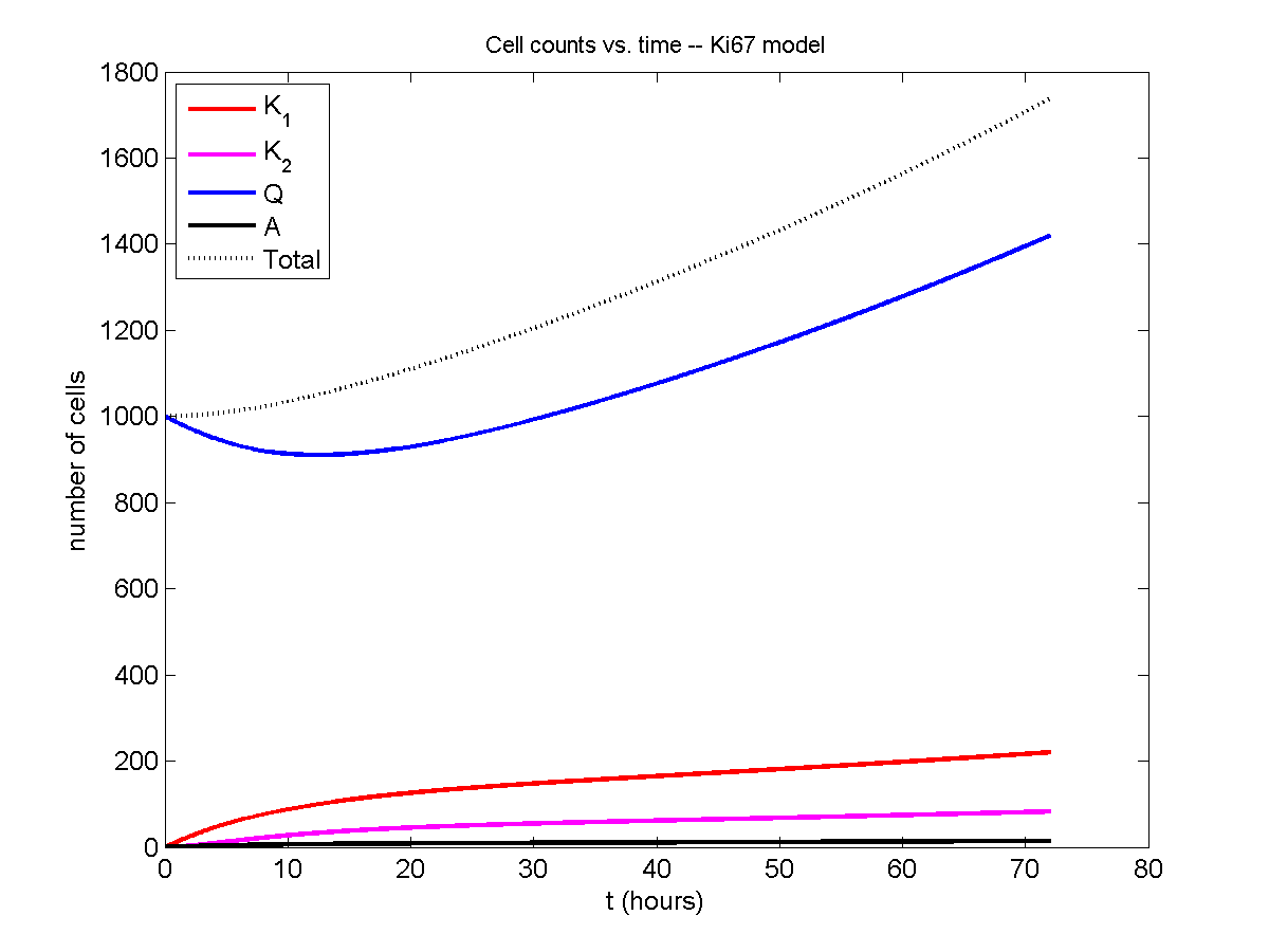
For the Ki67 model above, let \(\vec{N} = [K_1, K_2, Q, A]\). Then the linear system is
\[ \frac{d}{dt} \vec{N} = \begin{bmatrix} -\left( \frac{1}{T_1} + r_\mathrm{A} \right) & 0 & \frac{1}{T_\mathrm{Q}} & 0 \\ \frac{2}{T_1} & -\left( \frac{1}{T_2} + r_\mathrm{A} \right) & 0 & 0 \\ 0 & \frac{1}{T_2} & -\left( \frac{1}{T_\mathrm{Q}} + r_\mathrm{A} \right) & 0 \\ r_\mathrm{A} & r_\mathrm{A} & r_\mathrm{A} & -\frac{1}{T_\mathrm{A}} \end{bmatrix} \vec{N} .\]
(If we had written \( \vec{N} = [Q, K_1, K_2 , A] \), then the matrix above would have matched the general form.)
Some theoretical results
If \( M\) has eigenvalues \( \lambda_1 , \ldots \lambda_{n+1} \) and corresponding eigenvectors \( \vec{v}_1, \ldots , \vec{v}_{n+1} \), then the general solution is given by
\[ \vec{N}(t) = \sum_{i=1}^{n+1} c_i e^{ \lambda_i t } \vec{v}_i ,\] and if the initial cell counts are given by \( \vec{N}(0) \) and we write \( \vec{c} = [c_1, \ldots c_{n+1} ] \), we can obtain the coefficients by solving \[ \vec{N}(0) = [ \vec{v}_1 | \cdots | \vec{v}_{n+1} ]\vec{c} .\] In many cases, it turns out that all but one of the eigenvalues (say \( \lambda \) with corresponding eigenvector \(\vec{v}\)) are negative. In this case, all the other components of the solution decay away, and for long times, we have \[ \vec{N}(t) \approx c e^{ \lambda t } \vec{v} .\] This is incredibly useful, because it says that over long times, the fraction of cells in the \( i^\textrm{th} \) phase is given by \[ v_{i} / \sum_{j=1}^{n+1} v_{j}. \]
Matlab implementation (with the Ki67 model)
First, let’s set some parameters, to make this a little easier and reusable.
parameters.dt = 0.1; % 6 min = 0.1 hours
parameters.time_units = 'hour';
parameters.t_max = 3*24; % 3 days

parameters.K1.duration =  13;
parameters.K1.death_rate = 1.05e-3;
parameters.K1.initial = 0;

parameters.K2.duration = 2.5;
parameters.K2.death_rate = 1.05e-3;
parameters.K2.initial = 0;

parameters.Q.duration = 74.35 ;
parameters.Q.death_rate = 1.05e-3;
parameters.Q.initial = 1000;

parameters.A.duration = 8.6;
parameters.A.initial = 0;
Next, we write a function to read in the parameter values, construct the matrix (and all the data structures), find eigenvalues and eigenvectors, and create the theoretical solution. It also finds the positive eigenvalue to determine the long-time values.
function solution = Ki67_exact( parameters )
% allocate memory for the main outputs
solution.T = 0:parameters.dt:parameters.t_max;
solution.K1 = zeros( 1 , length(solution.T));
solution.K2 = zeros( 1 , length(solution.T));
solution.K = zeros( 1 , length(solution.T));
solution.Q = zeros( 1 , length(solution.T));
solution.A = zeros( 1 , length(solution.T));
solution.Live = zeros( 1 , length(solution.T));
solution.Total = zeros( 1 , length(solution.T));
% allocate memory for cell fractions
solution.AI = zeros(1,length(solution.T));
solution.KI1 = zeros(1,length(solution.T));
solution.KI2 = zeros(1,length(solution.T));
solution.KI = zeros(1,length(solution.T));
% get the main parameters
T1 = parameters.K1.duration;
r1A = parameters.K1.death_rate;
T2 = parameters.K2.duration;
r2A = parameters.K2.death_rate;
TQ = parameters.Q.duration;
rQA = parameters.Q.death_rate;
TA = parameters.A.duration;
% write out the mathematical model:
% d[Populations]/dt = Operator*[Populations]
Operator = [ -(1/T1 +r1A) , 0 , 1/TQ , 0; ...
2/T1 , -(1/T2 + r2A) ,0 , 0; ...
0 , 1/T2 , -(1/TQ + rQA) , 0; ...
r1A , r2A, rQA , -1/TA ];
% eigenvectors and eigenvalues
[V,D] = eig(Operator);
eigenvalues = diag(D);
% save the eigenvectors and eigenvalues in case you want them.
solution.V = V;
solution.D = D;
solution.eigenvalues = eigenvalues;
% initial condition
VecNow = [ parameters.K1.initial ; parameters.K2.initial ; ...
parameters.Q.initial ; parameters.A.initial ] ;
solution.K1(1) = VecNow(1);
solution.K2(1) = VecNow(2);
solution.Q(1) = VecNow(3);
solution.A(1) = VecNow(4);
solution.K(1) = solution.K1(1) + solution.K2(1);
solution.Live(1) = sum( VecNow(1:3) );
solution.Total(1) = sum( VecNow(1:4) );
solution.AI(1) = solution.A(1) / solution.Total(1);
solution.KI1(1) = solution.K1(1) / solution.Total(1);
solution.KI2(1) = solution.K2(1) / solution.Total(1);
solution.KI(1) = solution.KI1(1) + solution.KI2(1);
% now, get the coefficients to write the analytic solution
% [Populations] = c1*V(:,1)*exp( d(1,1)*t) + c2*V(:,2)*exp( d(2,2)*t ) +
% c3*V(:,3)*exp( d(3,3)*t) + c4*V(:,4)*exp( d(4,4)*t );
coeff = linsolve( V , VecNow );
% find the (hopefully one) positive eigenvalue.
% eigensolutions with negative eigenvalues decay,
% leaving this as the long-time behavior.
eigenvalues = diag(D);
n = find( real( eigenvalues ) &gt; 0 )
solution.long_time.KI1 = V(1,n) / sum( V(:,n) );
solution.long_time.KI2 = V(2,n) / sum( V(:,n) );
solution.long_time.QI = V(3,n) / sum( V(:,n) );
solution.long_time.AI = V(4,n) / sum( V(:,n) ) ;
solution.long_time.KI = solution.long_time.KI1 + solution.long_time.KI2;
% now, write out the solution at all the times
for i=2:length( solution.T )
% compact way to write the solution
VecExact = real( V*( coeff .* exp( eigenvalues*solution.T(i) ) ) );
solution.K1(i) = VecExact(1);
solution.K2(i) = VecExact(2);
solution.Q(i) = VecExact(3);
solution.A(i) = VecExact(4);
solution.K(i) = solution.K1(i) + solution.K2(i);
solution.Live(i) = sum( VecExact(1:3) );
solution.Total(i) = sum( VecExact(1:4) );
solution.AI(i) = solution.A(i) / solution.Total(i);
solution.KI1(i) = solution.K1(i) / solution.Total(i);
solution.KI2(i) = solution.K2(i) / solution.Total(i);
solution.KI(i) = solution.KI1(i) + solution.KI2(i);
end
return;
Now, let’s run it and see what this thing looks like:
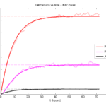
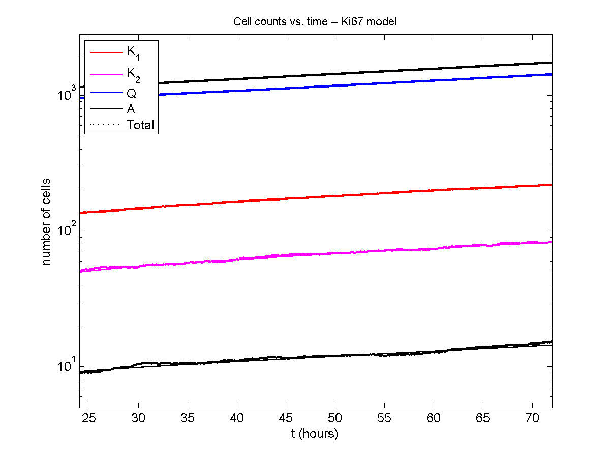
Next, we plot KI1, KI2, and AI versus time (solid curves), along with the theoretical long-time behavior (dashed curves). Notice how well it matches–it’s neat when theory works! :-)
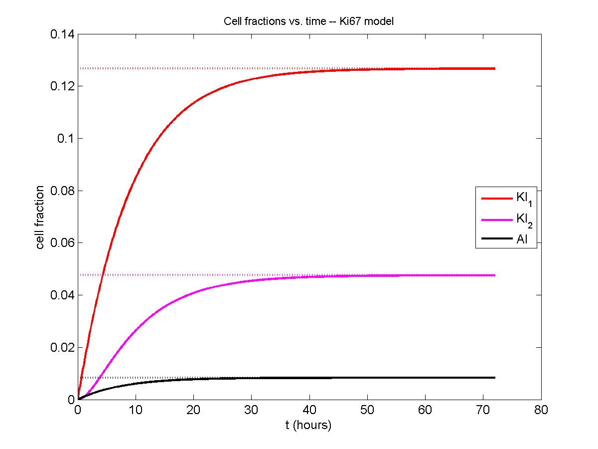
Some readers may recognize the long-time fractions: KI1 + KI2 = KI = 0.1743, and AI = 0.00833, very close to the DCIS patient values from our simulation study in Macklin et al. (2012) and improved calibration work in Hyun and Macklin (2013).
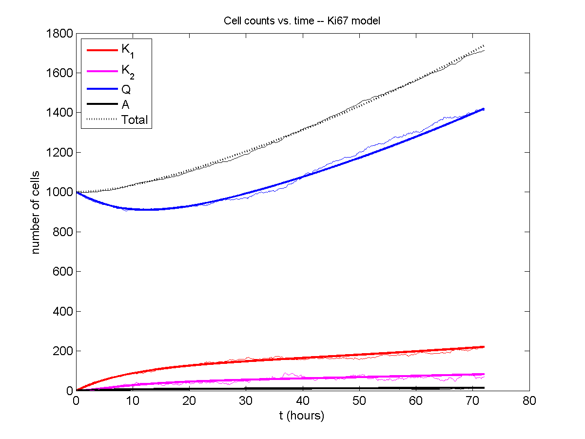
Comparing simulations and theory
I wrote a small Matlab program to implement the discrete model: start with 1000 cells in the \(Q\) phase, and in each time interval \([t,t+\Delta t]\), each cell “decides” whether to advance to the next phase, stay in the same phase, or apoptose. If we compare a single run against the theoretical curves, we see hints of a match:
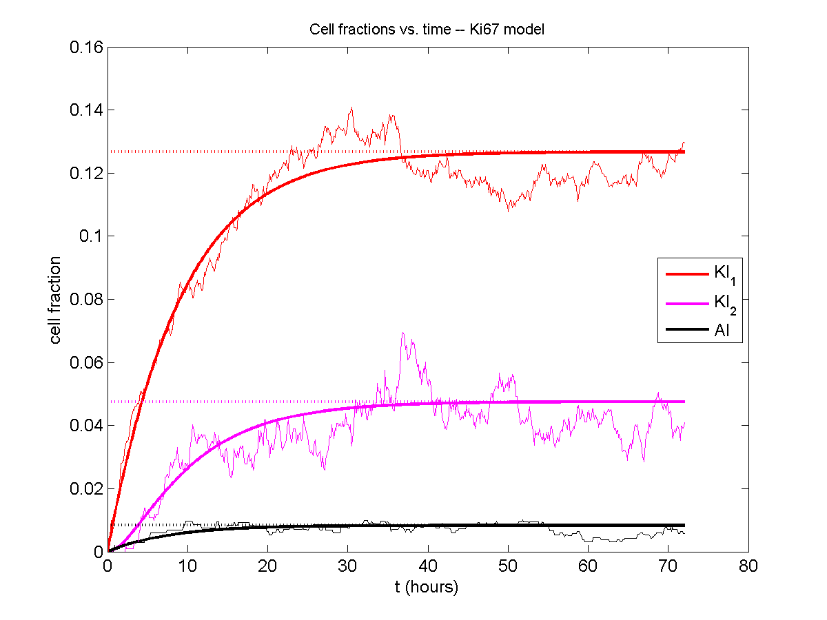
If we average 10 simulations and compare, the match is better:

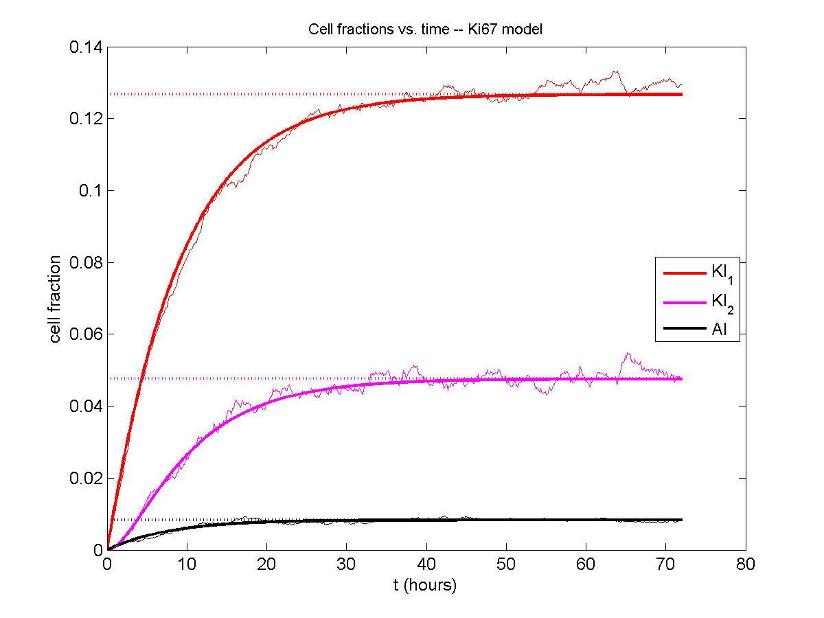
And lastly, if we average 100 simulations and compare, the curves are very difficult to tell apart:

Even in logarithmic space, it’s tough to tell these apart:
Code
The following matlab files (available here) can be used to reproduce this post:
- Ki67_exact.m
- The function defined above to create the exact solution using the eigenvalue/eignvector approach.
- Ki67_stochastic.m
- Runs a single stochastic simulation, using the supplied parameters.
- script.m
- Runs the theoretical solution first, creates plots, and then runs the stochastic model 100 times for comparison.
To make it all work, simply run “script” at the command prompt. Please note that it will generate some png files in its directory.
Closing thoughts
In this post, we showed a nice way to check a discrete model against theoretical behavior–both in short-term dynamics and long-time behavior. The same work should apply to validating many discrete models. However, when you add spatial effects (e.g., a cellular automaton model that won’t proliferate without an empty neighbor site), I wouldn’t expect a match. (But simulating cells that initially have a “salt and pepper”, random distribution should match this for early times.)
Moreover, models with deterministic phase durations (e.g., K1, K2, and A have fixed durations) aren’t consistent with the ODE model above, unless the cells they are each initialized with a random amount of “progress” in their initial phases. (Otherwise, the cells in each phase will run synchronized, and there will be fixed delays before cells transition to other phases.) Delay differential equations better describe such models. However, for long simulation times, the slopes of the sub-populations and the cell fractions should start to better and better match the ODE models.
Now that we have verified that the discrete model is performing as expected, we can have greater confidence in its predictions, and start using those predictions to assess the underlying models. In ODE and PDE models, you often validate the code on simpler problems where you have an analytical solution, and then move on to making simulation predictions in cases where you can’t solve analytically. Similarly, we can now move on to variants of the discrete model where we can’t as easily match ODE theory (e.g., time-varying rate parameters, spatial effects), but with the confidence that the phase transitions are working as they should.
DCIS modeling paper accepted
I am pleased to report that our paper has now been accepted. You can download the accepted preprint here. We also have a lot of supplementary material, including simulation movies, simulation datasets (for 0, 15, 30, adn 45 days of growth), and open source C++ code for postprocessing and visualization.
I discussed the results in detail here, but here’s the short version:
- We use a mechanistic, agent-based model of individual cancer cells growing in a duct. Cells are moved by adhesive and repulsive forces exchanged with other cells and the basement membrane. Cell phenotype is controlled by stochastic processes.
- We constrained all parameter expected to be relatively independent of patients by a careful analysis of the experimental biological and clinical literature.
- We developed the very first patient-specific calibration method, using clinically-accessible pathology. This is a key point in future patient-tailored predictions and surgical/therapeutic planning.
- The model made numerous quantitative predictions, such as:
- The tumor grows at a constant rate, between 7 to 10 mm/year. This is right in the middle of the range reported in the clinic.
- The tumor’s size in mammgraphy is linearly correlated with the post-surgical pathology size. When we linearly extrapolate our correlation across two orders of magnitude, it goes right through the middle of a cluster of 87 clinical data points.
- The tumor necrotic core has an age structuring: with oldest, calcified material in the center, and newest, most intact necrotic cells at the outer edge.
- The appearance of a “typical” DCIS duct cross-section varies with distance from the leading edge; all types of cross-sections predicted by our model are observed in patient pathology.
- The model also gave new insight on the underlying biology of breast cancer, such as:
- The split between the viable rim and necrotic core (observed almost universally in pathology) is not just an artifact, but an actual biomechanical effect from fast necrotic cell lysis.
- The constant rate of tumor growth arises from the biomechanical stress relief provided by lysing necrotic cells. This points to the critical role of intracellular and intra-tumoral water transport in determining the qualitative and quantitative behavior of tumors.
- Pyknosis (nuclear degradation in necrotic cells), must occur at a time scale between that of cell lysis (on the order of hours) and cell calcification (on the order of weeks).
- The current model cannot explain the full spectrum of calcification types; other biophysics, such as degradation over a long, 1-2 month time scale, must be at play.
Now hiring: Postdoctoral Researcher
I just posted a job opportunity for a postdoctoral researcher for computational modeling of breast, prostate, and metastatic cancer, with a heavy emphasis on calibrating (and validating!) to in vitro, in vivo, and clinical data.
If you’re a talented computational modeler and have a passion for applying mathematics to make a difference in clinical care, please read the job posting and apply!
(Note: Interested students in the Los Angeles/Orange County area may want to attend my applied math seminar talk at UCI next week to learn more about this work.)
MMCL welcomes Gianluca D’Antonio
The Macklin Math Cancer Lab is pleased to welcome Gianluca D’Antonio, a M.S. student of Luigi Preziosi and mathematician from Politecnico di Torino. Gianluca, who brings with him a wealth of expertise in biomechanics modeling, will spend 6 months at CAMM at the Keck School of Medicine of USC to model basement membrane deformation by growing tumors, biomechanical feedback between the stroma and growing tumors, and related problems. Gianluca’s interests and expertise fit very nicely into our broader vision of mechanistic cancer modeling, as well as USC / CAMM’s focus on applying the physical sciences to cancer (as part of the USC-led PSOC).
He is our first international visiting scholar, and we’re very excited for the multidisciplinary work we will accomplish together! So, please join us in welcoming Gianluca!
PSOC Short Course on Multidisciplinary Cancer Modeling
Next Monday (October 17, 2011), the USC-led Physical Sciences Oncology Center / CAMM will host a short course on multidisciplinary cancer modeling, combining the expertise of biologists, oncologists, and physical scientists. I’ll attach a PDF flyer of the schedule below. I am giving a talk during “Session II – The Physicist Perspective on Cancer.” I will focus on tailoring mathematical models from the ground up to clinical data from individual patients, with an emphasis on using computational models to make testable clinical predictions, and using these models a platforms to generate hypotheses on cancer biology.
The response to our short course has been overwhelming (in a good way), with around 200 registrants! So, registration is unfortunately closed at this time. However, the talks will be broadcast live via a webcast. The link and login details are in the PDF below. I hope to see you there! — Paul
Agenda
7:00 am – 8:25 am : Registration, breakfast, and opening comments, etc.
David B. Agus, M.D. (Director of USC CAMM)
W. Daniel Hillis, Ph.D. (PI of USC PSOC, Applied Minds)
Larry A. Nagahara (NCI PSOC Program Director)
8:30 am – 10:15 am : Session I – Cancer Biology and the Cancer Genome
Paul Mischel, UCLA – The Biology of Cancer from Cell to Patient, Oncogenesis to Therapeutic Response
Matteo Pellegrini, UCLA – Evolution in Cancer
Mitchelll Gross, USC – Historical Perspective on Cancer Diagnosis and Treatment
10:30 am – 12:15 pm : Session II – The Physicist Perspective on Cancer
Dan Ruderman, USC – Cancer as a Multi-scale Problem
Paul Macklin, USC – Computational Models of Cancer Growth
Tom Tombrello, Cal-Tech – Perspective: Big Problems in Physics vs. Cancer
1:45 pm. – 3:10 pm : Session III – Novel Measurement Platforms & Data Management & Integration
Michelle Povinelli, USC – The Role of Novel Microdevices in Dissecting Cellular Phenomena
Carl Kesselman, USC – Data Management & Integration Challenges in Interdisciplinary Studies
3:10 pm – 3:40 pm : Session IV – Creativity in Research at the Interface between the Life and Physical Sciences
‘Fireside Chat’ David Agus and Danny Hillis, USC
4:00 pm – 5:00 pm : Capstone – Keynote Speaker
Tim Walsh, Game Inventor, Keynote Speaker
5:30 pm – 8:00 pm : Poster Session and Reception