Category: cellular automaton
Coarse-graining discrete cell cycle models
Introduction
One observation that often goes underappreciated in computational biology discussions is that a computational model is often a model of a model of a model of biology: that is, it’s a numerical approximation (a model) of a mathematical model of an experimental model of a real-life biological system. Thus, there are three big places where a computational investigation can fall flat:
- The experimental model may be a bad choice for the disease or process (not our fault).
- Second, the mathematical model of the experimental system may have flawed assumptions (something we have to evaluate).
- The numerical implementation may have bugs or otherwise be mathematically inconsistent with the mathematical model.
Critically, you can’t use simulations to evaluate the experimental model or the mathematical model until you verify that the numerical implementation is consistent with the mathematical model, and that the numerical solution converges as \( \Delta t\) and \( \Delta x \) shrink to zero.
There are numerous ways to accomplish this, but ideally, it boils down to having some analytical solutions to the mathematical model, and comparing numerical solutions to these analytical or theoretical results. In this post, we’re going to walk through the math of analyzing a typical type of discrete cell cycle model.
Discrete model
Suppose we have a cell cycle model consisting of phases \(P_1, P_2, \ldots P_n \), where cells in the \(P_i\) phase progress to the \(P_{i+1}\) phase after a mean waiting time of \(T_i\), and cells leaving the \(P_n\) phase divide into two cells in the \(P_1\) phase. Assign each cell agent \(k\) a current phenotypic phase \( S_k(t) \). Suppose also that each phase \( i \) has a death rate \( d_i \), and that cells persist for on average \( T_\mathrm{A} \) time in the dead state before they are removed from the simulation.
The mean waiting times \( T_i \) are equivalent to transition rates \( r_i = 1 / T_i \) (Macklin et al. 2012). Moreover, for any time interval \( [t,t+\Delta t] \), both are equivalent to a transition probability of
\[ \mathrm{Prob}\Bigl( S_k(t+\Delta t) = P_{i+1} | S(t) = P_i \Bigr) = 1 – e^{ -r_i \Delta t } \approx r_i \Delta t = \frac{ \Delta t}{ T_i}. \] In many discrete models (especially cellular automaton models) with fixed step sizes \( \Delta t \), models are stated in terms of transition probabilities \( p_{i,i+1} \), which we see are equivalent to the work above with \( p_{i,i+1} = r_i \Delta t = \Delta t / T_i \), allowing us to tie mathematical model forms to biological, measurable parameters. We note that each \(T_i\) is the average duration of the \( P_i \) phase.
Concrete example: a Ki67 Model
Ki-67 is a nuclear protein that is expressed through much of the cell cycle, including S, G2, M, and part of G1 after division. It is used very commonly in pathology to assess proliferation, particularly in cancer. See the references and discussion in (Macklin et al. 2012). In Macklin et al. (2012), we came up with a discrete cell cycle model to match Ki-67 data (along with cleaved Caspase-3 stains for apoptotic cells). Let’s summarize the key parts here.
Each cell agent \(i\) has a phase \(S_i(t)\). Ki67- cells are quiescent (phase \(Q\), mean duration \( T_\mathrm{Q} \)), and they can enter the Ki67+ \(K_1\) phase (mean duration \(T_1\)). When \( K_1 \) cells leave their phase, they divide into two Ki67+ daughter cells in the \( K_2 \) phase with mean duration \( T_2 \). When cells exit \( K_2 \), they return to \( Q \). Cells in any phase can become apoptotic (enter the \( A \) phase with mean duration \( T_\mathrm{A} \)), with death rate \( r_\mathrm{A} \).
Coarse-graining to an ODE model
If each phase \(i\) has a death rate \(d_i\), if \( N_i(t) \) denotes the number of cells in the \( P_i \) phase at time \( t\), and if \( A(t) \) is the number of dead (apoptotic) cells at time \( t\), then on average, the number of cells in the \( P_i \) phase at the next time step is given by
\[ N_i(t+\Delta t) = N_i(t) + N_{i-1}(t) \cdot \left[ \textrm{prob. of } P_{i-1} \rightarrow P_i \textrm{ transition} \right] – N_i(t) \cdot \left[ \textrm{prob. of } P_{i} \rightarrow P_{i+1} \textrm{ transition} \right] \] \[ – N_i(t) \cdot \left[ \textrm{probability of death} \right] \] By the work above, this is:
\[ N_i(t+\Delta t) \approx N_i(t) + N_{i-1}(t) r_{i-1} \Delta t – N_i(t) r_i \Delta t – N_i(t) d_i \Delta t , \] or after shuffling terms and taking the limit as \( \Delta t \downarrow 0\), \[ \frac{d}{dt} N_i(t) = r_{i-1} N_{i-1}(t) – \left( r_i + d_i \right) N_i(t). \] Continuing this analysis, we obtain a linear system:
\[ \frac{d}{dt}{ \vec{N} } = \begin{bmatrix} -(r_1+d_1) & 0 & \cdots & 0 & 2r_n & 0 \\ r_1 & -(r_2+d_2) & 0 & \cdots & 0 & 0 \\ 0 & r_2 & -(r_3+d_3) & 0 & \cdots & 0 \\ & & \ddots & & \\0&\cdots&0 &r_{n-1} & -(r_n+d_n) & 0 \\ d_1 & d_2 & \cdots & d_{n-1} & d_n & -\frac{1}{T_\mathrm{A}} \end{bmatrix}\vec{N} = M \vec{N}, \] where \( \vec{N}(t) = [ N_1(t), N_2(t) , \ldots , N_n(t) , A(t) ] \).
For the Ki67 model above, let \(\vec{N} = [K_1, K_2, Q, A]\). Then the linear system is
\[ \frac{d}{dt} \vec{N} = \begin{bmatrix} -\left( \frac{1}{T_1} + r_\mathrm{A} \right) & 0 & \frac{1}{T_\mathrm{Q}} & 0 \\ \frac{2}{T_1} & -\left( \frac{1}{T_2} + r_\mathrm{A} \right) & 0 & 0 \\ 0 & \frac{1}{T_2} & -\left( \frac{1}{T_\mathrm{Q}} + r_\mathrm{A} \right) & 0 \\ r_\mathrm{A} & r_\mathrm{A} & r_\mathrm{A} & -\frac{1}{T_\mathrm{A}} \end{bmatrix} \vec{N} .\]
(If we had written \( \vec{N} = [Q, K_1, K_2 , A] \), then the matrix above would have matched the general form.)
Some theoretical results
If \( M\) has eigenvalues \( \lambda_1 , \ldots \lambda_{n+1} \) and corresponding eigenvectors \( \vec{v}_1, \ldots , \vec{v}_{n+1} \), then the general solution is given by
\[ \vec{N}(t) = \sum_{i=1}^{n+1} c_i e^{ \lambda_i t } \vec{v}_i ,\] and if the initial cell counts are given by \( \vec{N}(0) \) and we write \( \vec{c} = [c_1, \ldots c_{n+1} ] \), we can obtain the coefficients by solving \[ \vec{N}(0) = [ \vec{v}_1 | \cdots | \vec{v}_{n+1} ]\vec{c} .\] In many cases, it turns out that all but one of the eigenvalues (say \( \lambda \) with corresponding eigenvector \(\vec{v}\)) are negative. In this case, all the other components of the solution decay away, and for long times, we have \[ \vec{N}(t) \approx c e^{ \lambda t } \vec{v} .\] This is incredibly useful, because it says that over long times, the fraction of cells in the \( i^\textrm{th} \) phase is given by \[ v_{i} / \sum_{j=1}^{n+1} v_{j}. \]
Matlab implementation (with the Ki67 model)
First, let’s set some parameters, to make this a little easier and reusable.
parameters.dt = 0.1; % 6 min = 0.1 hours
parameters.time_units = 'hour';
parameters.t_max = 3*24; % 3 days

parameters.K1.duration =  13;
parameters.K1.death_rate = 1.05e-3;
parameters.K1.initial = 0;

parameters.K2.duration = 2.5;
parameters.K2.death_rate = 1.05e-3;
parameters.K2.initial = 0;

parameters.Q.duration = 74.35 ;
parameters.Q.death_rate = 1.05e-3;
parameters.Q.initial = 1000;

parameters.A.duration = 8.6;
parameters.A.initial = 0;
Next, we write a function to read in the parameter values, construct the matrix (and all the data structures), find eigenvalues and eigenvectors, and create the theoretical solution. It also finds the positive eigenvalue to determine the long-time values.
function solution = Ki67_exact( parameters )

% allocate memory for the main outputs

solution.T = 0:parameters.dt:parameters.t_max;
solution.K1 = zeros( 1 , length(solution.T));
solution.K2 = zeros( 1 , length(solution.T));
solution.K = zeros( 1 , length(solution.T));
solution.Q = zeros( 1 , length(solution.T));
solution.A = zeros( 1 , length(solution.T));
solution.Live = zeros( 1 , length(solution.T));
solution.Total = zeros( 1 , length(solution.T));

% allocate memory for cell fractions

solution.AI = zeros(1,length(solution.T));
solution.KI1 = zeros(1,length(solution.T));
solution.KI2 = zeros(1,length(solution.T));
solution.KI = zeros(1,length(solution.T));

% get the main parameters

T1 = parameters.K1.duration;
r1A = parameters.K1.death_rate;

T2 = parameters.K2.duration;
r2A = parameters.K2.death_rate;

TQ = parameters.Q.duration;
rQA = parameters.Q.death_rate;

TA = parameters.A.duration;

% write out the mathematical model:
% d[Populations]/dt = Operator*[Populations]

Operator = [ -(1/T1 +r1A) , 0 , 1/TQ , 0; ...
    2/T1 , -(1/T2 + r2A) ,0 , 0; ...
    0 , 1/T2 , -(1/TQ + rQA) , 0; ...
    r1A , r2A, rQA , -1/TA ];

% eigenvectors and eigenvalues

[V,D] = eig(Operator);
eigenvalues = diag(D);

% save the eigenvectors and eigenvalues in case you want them.

solution.V = V;
solution.D = D;
solution.eigenvalues = eigenvalues;

% initial condition

VecNow = [ parameters.K1.initial ; parameters.K2.initial ; ...
    parameters.Q.initial ; parameters.A.initial ] ;
solution.K1(1) = VecNow(1);
solution.K2(1) = VecNow(2);
solution.Q(1) = VecNow(3);
solution.A(1) = VecNow(4);
solution.K(1) = solution.K1(1) + solution.K2(1);
solution.Live(1) = sum( VecNow(1:3) );
solution.Total(1) = sum( VecNow(1:4) );

solution.AI(1) = solution.A(1) / solution.Total(1);
solution.KI1(1) = solution.K1(1) / solution.Total(1);
solution.KI2(1) = solution.K2(1) / solution.Total(1);
solution.KI(1) = solution.KI1(1) + solution.KI2(1);

% now, get the coefficients to write the analytic solution
% [Populations] = c1*V(:,1)*exp( d(1,1)*t) + c2*V(:,2)*exp( d(2,2)*t ) +
%                 c3*V(:,3)*exp( d(3,3)*t) + c4*V(:,4)*exp( d(4,4)*t );

coeff = linsolve( V , VecNow );

% find the (hopefully one) positive eigenvalue.
% eigensolutions with negative eigenvalues decay,
% leaving this as the long-time behavior.

eigenvalues = diag(D);
n = find( real( eigenvalues ) > 0 )
solution.long_time.KI1 = V(1,n) / sum( V(:,n) );
solution.long_time.KI2 = V(2,n) / sum( V(:,n) );
solution.long_time.QI = V(3,n) / sum( V(:,n) );
solution.long_time.AI = V(4,n) / sum( V(:,n) ) ;
solution.long_time.KI = solution.long_time.KI1 + solution.long_time.KI2;

% now, write out the solution at all the times
for i=2:length( solution.T )
    % compact way to write the solution
    VecExact = real( V*( coeff .* exp( eigenvalues*solution.T(i) ) ) );

    solution.K1(i) = VecExact(1);
    solution.K2(i) = VecExact(2);
    solution.Q(i) = VecExact(3);
    solution.A(i) = VecExact(4);
    solution.K(i) = solution.K1(i) + solution.K2(i);
    solution.Live(i) = sum( VecExact(1:3) );
    solution.Total(i) = sum( VecExact(1:4) );

    solution.AI(i) = solution.A(i) / solution.Total(i);
    solution.KI1(i) = solution.K1(i) / solution.Total(i);
    solution.KI2(i) = solution.K2(i) / solution.Total(i);
    solution.KI(i) = solution.KI1(i) + solution.KI2(i);
end

return;
Now, let’s run it and see what this thing looks like:
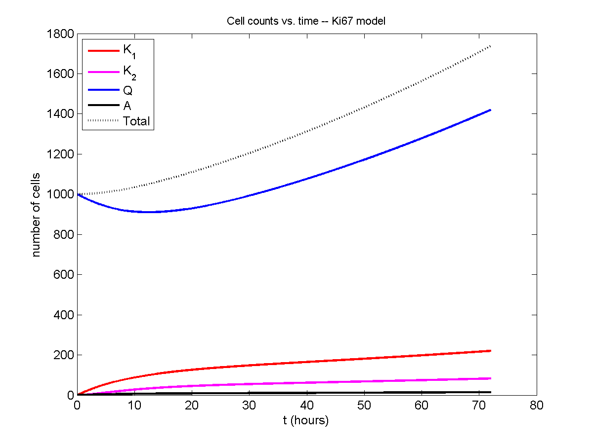
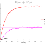
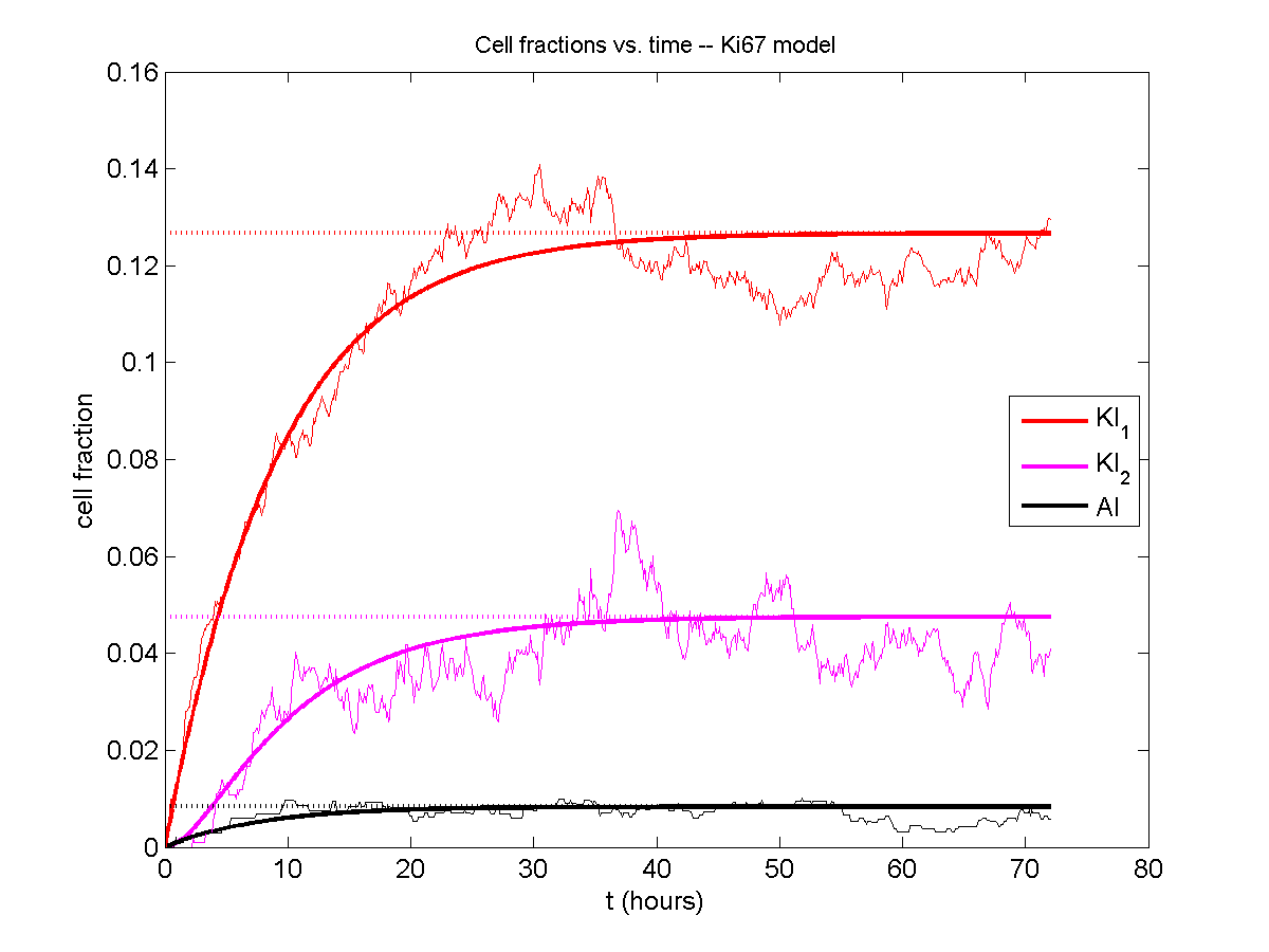
Next, we plot KI1, KI2, and AI versus time (solid curves), along with the theoretical long-time behavior (dashed curves). Notice how well it matches–it’s neat when theory works! :-)
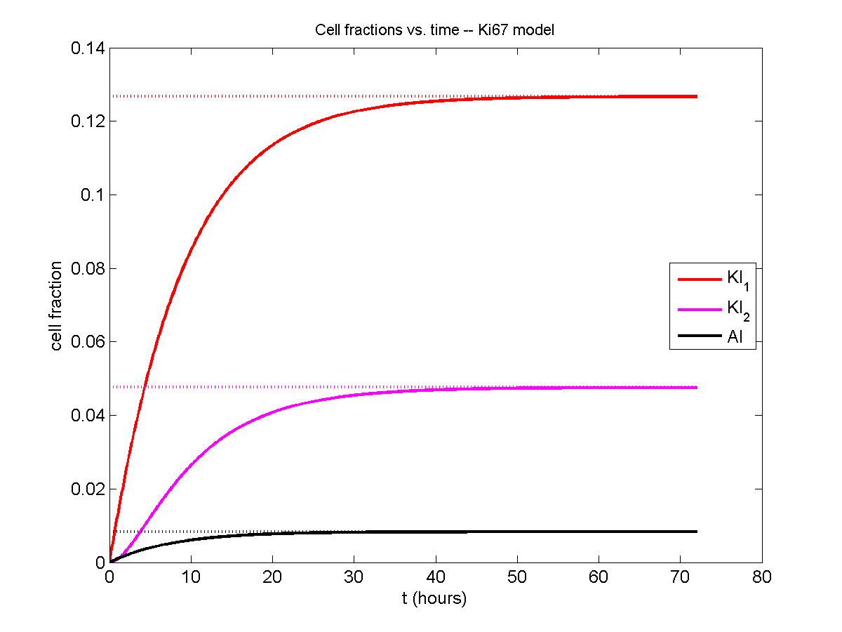
Some readers may recognize the long-time fractions: KI1 + KI2 = KI = 0.1743, and AI = 0.00833, very close to the DCIS patient values from our simulation study in Macklin et al. (2012) and improved calibration work in Hyun and Macklin (2013).
Comparing simulations and theory
I wrote a small Matlab program to implement the discrete model: start with 1000 cells in the \(Q\) phase, and in each time interval \([t,t+\Delta t]\), each cell “decides” whether to advance to the next phase, stay in the same phase, or apoptose. If we compare a single run against the theoretical curves, we see hints of a match:
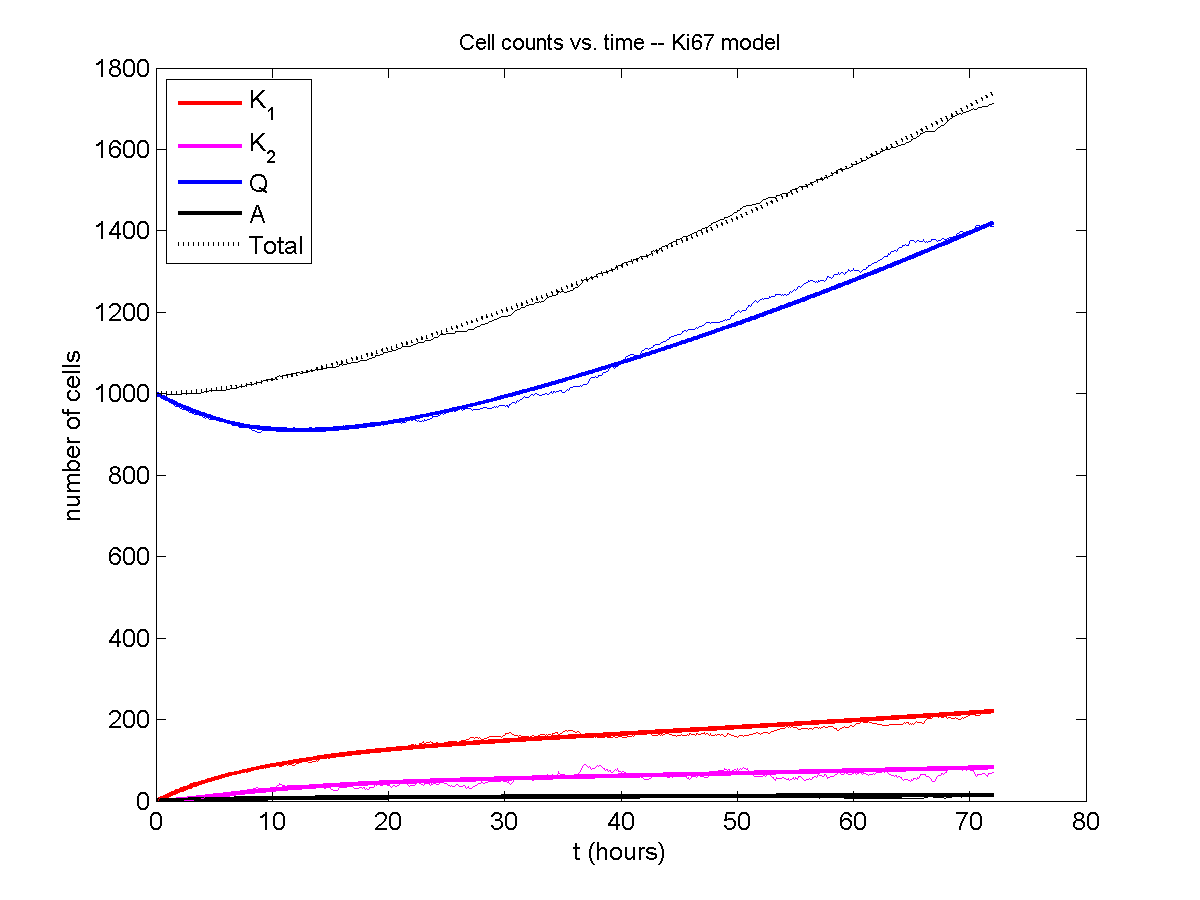
If we average 10 simulations and compare, the match is better:

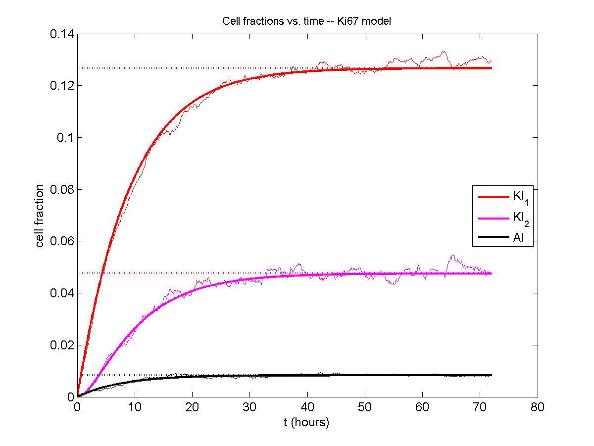
And lastly, if we average 100 simulations and compare, the curves are very difficult to tell apart:

Even in logarithmic space, it’s tough to tell these apart:
Code
The following matlab files (available here) can be used to reproduce this post:
- Ki67_exact.m
- The function defined above to create the exact solution using the eigenvalue/eignvector approach.
- Ki67_stochastic.m
- Runs a single stochastic simulation, using the supplied parameters.
- script.m
- Runs the theoretical solution first, creates plots, and then runs the stochastic model 100 times for comparison.
To make it all work, simply run “script” at the command prompt. Please note that it will generate some png files in its directory.
Closing thoughts
In this post, we showed a nice way to check a discrete model against theoretical behavior–both in short-term dynamics and long-time behavior. The same work should apply to validating many discrete models. However, when you add spatial effects (e.g., a cellular automaton model that won’t proliferate without an empty neighbor site), I wouldn’t expect a match. (But simulating cells that initially have a “salt and pepper”, random distribution should match this for early times.)
Moreover, models with deterministic phase durations (e.g., K1, K2, and A have fixed durations) aren’t consistent with the ODE model above, unless the cells they are each initialized with a random amount of “progress” in their initial phases. (Otherwise, the cells in each phase will run synchronized, and there will be fixed delays before cells transition to other phases.) Delay differential equations better describe such models. However, for long simulation times, the slopes of the sub-populations and the cell fractions should start to better and better match the ODE models.
Now that we have verified that the discrete model is performing as expected, we can have greater confidence in its predictions, and start using those predictions to assess the underlying models. In ODE and PDE models, you often validate the code on simpler problems where you have an analytical solution, and then move on to making simulation predictions in cases where you can’t solve analytically. Similarly, we can now move on to variants of the discrete model where we can’t as easily match ODE theory (e.g., time-varying rate parameters, spatial effects), but with the confidence that the phase transitions are working as they should.
Building a Cellular Automaton Model Using BioFVM
Note: This is part of a series of “how-to” blog posts to help new users and developers of BioFVM. See below for guides to setting up a C++ compiler in Windows or OSX.
What you’ll need
- A working C++ development environment with support for OpenMP. See these prior tutorials if you need help.
- A download of BioFVM, available at http://BioFVM.MathCancer.org and http://BioFVM.sf.net. Use Version 1.1.4 or later.
- The source code for this project (see below).
Matlab or Octave for visualization. Matlab might be available for free at your university. Octave is open source and available from a variety of sources.
Our modeling task
We will implement a basic 3-D cellular automaton model of tumor growth in a well-mixed fluid, containing oxygen pO2 (mmHg) and a drug c (e.g., doxorubicin, μM), inspired by modeling by Alexander Anderson, Heiko Enderling, Jan Poleszczuk, Gibin Powathil, and others. (I highly suggest seeking out the sophisticated cellular automaton models at Moffitt’s Integrated Mathematical Oncology program!) This example shows you how to extend BioFVM into a new cellular automaton model. I’ll write a similar post on how to add BioFVM into an existing cellular automaton model, which you may already have available.
Tumor growth will be driven by oxygen availability. Tumor cells can be live, apoptotic (going through energy-dependent cell death, or necrotic (undergoing death from energy collapse). Drug exposure can both trigger apoptosis and inhibit cell cycling. We will model this as growth into a well-mixed fluid, with pO2 = 38 mmHg (about 5% oxygen: a physioxic value) and c = 5 μM.
Mathematical model
As a cellular automaton model, we will divide 3-D space into a regular lattice of voxels, with length, width, and height of 15 μm. (A typical breast cancer cell has radius around 9-10 μm, giving a typical volume around 3.6×103 μm3. If we make each lattice site have the volume of one cell, this gives an edge length around 15 μm.)
In voxels unoccupied by cells, we approximate a well-mixed fluid with Dirichlet nodes, setting pO2 = 38 mmHg, and initially setting c = 0. Whenever a cell dies, we replace it with an empty automaton, with no Dirichlet node. Oxygen and drug follow the typical diffusion-reaction equations:
\[ \frac{ \partial \textrm{pO}_2 }{\partial t} = D_\textrm{oxy} \nabla^2 \textrm{pO}_2 – \lambda_\textrm{oxy} \textrm{pO}_2 – \sum_{ \textrm{cells} i} U_{i,\textrm{oxy}} \textrm{pO}_2 \]
\[ \frac{ \partial c}{ \partial t } = D_c \nabla^2 c – \lambda_c c – \sum_{\textrm{cells }i} U_{i,c} c \]
where each uptake rate is applied across the cell’s volume. We start the treatment by setting c = 5 μM on all Dirichlet nodes at t = 504 hours (21 days). For simplicity, we do not model drug degradation (pharmacokinetics), to approximate the in vitro conditions.
In any time interval [t,t+Δt], each live tumor cell i has a probability pi,D of attempting division, probability pi,A of apoptotic death, and probability pi,N of necrotic death. (For simplicity, we ignore motility in this version.) We relate these to the birth rate bi, apoptotic death rate di,A, and necrotic death rate di,N by the linearized equations (from Macklin et al. 2012):
\[ \textrm{Prob} \Bigl( \textrm{cell } i \textrm{ becomes apoptotic in } [t,t+\Delta t] \Bigr) = 1 – \textrm{exp}\Bigl( -d_{i,A}(t) \Delta t\Bigr) \approx d_{i,A}\Delta t \]
\[ \textrm{Prob} \Bigl( \textrm{cell } i \textrm{ attempts division in } [t,t+\Delta t] \Bigr) = 1 – \textrm{exp}\Bigl( -b_i(t) \Delta t\Bigr) \approx b_{i}\Delta t \]
\[ \textrm{Prob} \Bigl( \textrm{cell } i \textrm{ becomes necrotic in } [t,t+\Delta t] \Bigr) = 1 – \textrm{exp}\Bigl( -d_{i,N}(t) \Delta t\Bigr) \approx d_{i,N}\Delta t \]
\[ \textrm{Prob} \Bigl( \textrm{dead cell } i \textrm{ lyses in } [t,t+\Delta t] \Bigr) = 1 – \textrm{exp}\Bigl( -\frac{1}{T_{i,D}} \Delta t\Bigr) \approx \frac{ \Delta t}{T_{i,D}} \]
(Illustrative) parameter values
We use Doxy = 105 μm2/min (Ghaffarizadeh et al. 2016), and we set Ui,oxy = 20 min-1 (to give an oxygen diffusion length scale of about 70 μm, with steeper gradients than our typical 100 μm length scale). We set λoxy = 0.01 min-1 for a 1 mm diffusion length scale in fluid.
We set Dc = 300 μm2/min, and Uc = 7.2×10⁻³ min-1 (Dc from Weinberg et al. (2007), and Ui,c twice as large as the reference value in Weinberg et al. (2007) to get a smaller diffusion length scale of about 204 μm). We set λc = 3.6×10⁻⁵ min-1 to give a drug diffusion length scale of about 2.9 mm in fluid.
We use TD = 8.6 hours for apoptotic cells, and TD = 60 days for necrotic cells (Macklin et al., 2013). However, note that necrotic and apoptotic cells lose volume quickly, so one may want to revise those time scales to match the point where a cell loses 90% of its volume.
Functional forms for the birth and death rates
We model pharmacodynamics with an area-under-the-curve (AUC) type formulation. If c(t) is the drug concentration at any cell i‘s location at time t, then let its integrated exposure Ei(t) be
\[ E_i(t) = \int_0^t c(s) \: ds \]
and we model its response with a Hill function
\[ R_i(t) = \frac{ E_i^h(t) }{ \alpha_i^h + E_i^h(t) }, \]
where h is the drug’s Hill exponent for the cell line, and α is the exposure for a half-maximum effect.
We model the microenvironment-dependent birth rate by:
\[ b_i(t) = \left\{ \begin{array}{lr} b_{i,P} \left( 1 – \eta_i R_i(t) \right) & \textrm{ if } \textrm{pO}_{2,P} < \textrm{pO}_2 \\ \\ b_{i,P} \left( \frac{\textrm{pO}_{2}-\textrm{pO}_{2,N}}{\textrm{pO}_{2,P}-\textrm{pO}_{2,N}}\right) \Bigl( 1 – \eta_i R_i(t) \Bigr) & \textrm{ if } \textrm{pO}_{2,N} < \textrm{pO}_2 \le \textrm{pO}_{2,P} \\ \\ 0 & \textrm{ if } \textrm{pO}_2 \le \textrm{pO}_{2,N}\end{array} \right. \]
where pO2,P is the physioxic oxygen value (38 mmHg), and pO2,N is a necrotic threshold (we use 5 mmHg), and 0 < η < 1 the drug’s birth inhibition. (A fully cytostatic drug has η = 1.)
We model the microenvironment-dependent apoptosis rate by:
\[ d_{i,A}(t) = d_{i,A}^* + \Bigl( d_{i,A}^\textrm{max} – d_{i,A}^* \Bigr) R_i(t) \]
\[ d_{i,N}(t) = \left\{ \begin{array}{lr} 0 & \textrm{ if } \textrm{pO}_{2,N} < \textrm{pO}_{2} \\ \\ d_{i,N}^* & \textrm{ if } \textrm{pO}_{2} \le \textrm{pO}_{2,N} \end{array}\right. \]
(Illustrative) parameter values
We use bi,P = 0.05 hour-1 (for a 20 hour cell cycle in physioxic conditions), di,A* = 0.01 bi,P, and di,N* = 0.04 hour-1 (so necrotic cells survive around 25 hours in low oxygen conditions).
We set α = 30 μM*hour (so that cells reach half max response after 6 hours’ exposure at a maximum concentration c = 5 μM), h = 2 (for a smooth effect), η = 0.25 (so that the drug is partly cytostatic), and di,Amax = 0.1 hour^-1 (so that cells survive about 10 hours after reaching maximum response).
Building the Cellular Automaton Model in BioFVM
BioFVM already includes Basic_Agents for cell-based substrate sources and sinks. We can extend these basic agents into full-fledged automata, and then arrange them in a lattice to create a full cellular automata model. Let’s sketch that out now.
Extending Basic_Agents to Automata
The main idea here is to define an Automaton class which extends (and therefore includes) the Basic_Agent class. This will give each Automaton full access to the microenvironment defined in BioFVM, including the ability to secrete and uptake substrates. We also make sure each Automaton “knows” which microenvironment it lives in (contains a pointer pMicroenvironment), and “knows” where it lives in the cellular automaton lattice. (More on that in the following paragraphs.)
So, as a schematic (just sketching out the most important members of the class):
class Standard_Data; // define per-cell biological data, such as phenotype,
	// cell cycle status, etc..
class Custom_Data; // user-defined custom data, specific to a model.

class Automaton : public Basic_Agent
{
	private:
		Microenvironment* pMicroenvironment;

		CA_Mesh* pCA_mesh;
		int voxel_index;

	protected:
	public:
		// neighbor connectivity information
		std::vector<Automaton*> neighbors;
		std::vector<double> neighbor_weights;

		Standard_Data standard_data;
		void (*current_state_rule)( Automaton& A , double );

		Automaton();
		void copy_parameters( Standard_Data& SD  );
		void overwrite_from_automaton( Automaton& A );

		void set_cellular_automaton_mesh( CA_Mesh* pMesh );
		CA_Mesh* get_cellular_automaton_mesh( void ) const;

		void set_voxel_index( int );
		int get_voxel_index( void ) const;

		void set_microenvironment( Microenvironment* pME );
		Microenvironment* get_microenvironment( void );

		// standard state changes
		bool attempt_division( void );
		void become_apoptotic( void );
		void become_necrotic( void );
		void perform_lysis( void );

		// things the user needs to define

		Custom_Data custom_data;

		// use this rule to add custom logic
		void (*custom_rule)( Automaton& A , double);
};
So, the Automaton class includes everything in the Basic_Agent class, some Standard_Data (things like the cell state and phenotype, and per-cell settings), (user-defined) Custom_Data, basic cell behaviors like attempting division into an empty neighbor lattice site, and user-defined custom logic that can be applied to any automaton. To avoid lots of switch/case and if/then logic, each Automaton has a function pointer for its current activity (current_state_rule), which can be overwritten any time.
Each Automaton also has a list of neighbor Automata (their memory addresses), and weights for each of these neighbors. Thus, you can distance-weight the neighbors (so that corner elements are farther away), and very generalized neighbor models are possible (e.g., all lattice sites within a certain distance). When updating a cellular automaton model, such as to kill a cell, divide it, or move it, you leave the neighbor information alone, and copy/edit the information (standard_data, custom_data, current_state_rule, custom_rule). In many ways, an Automaton is just a bucket with a cell’s information in it.
Note that each Automaton also “knows” where it lives (pMicroenvironment and voxel_index), and knows what CA_Mesh it is attached to (more below).
Connecting Automata into a Lattice
An automaton by itself is lost in the world–it needs to link up into a lattice organization. Here’s where we define a CA_Mesh class, to hold the entire collection of Automata, setup functions (to match to the microenvironment), and two fundamental operations at the mesh level: copying automata (for cell division), and swapping them (for motility). We have provided two functions to accomplish these tasks, while automatically keeping the indexing and BioFVM functions correctly in sync. Here’s what it looks like:
class CA_Mesh{
	private:
		Microenvironment* pMicroenvironment;
		Cartesian_Mesh* pMesh;

		std::vector<Automaton> automata;
		std::vector<int> iteration_order;
	protected:
	public:
		CA_Mesh();

		// setup to match a supplied microenvironment
		void setup( Microenvironment& M );
		// setup to match the default microenvironment
		void setup( void );

		int number_of_automata( void ) const;

		void randomize_iteration_order( void );

		void swap_automata( int i, int j );
		void overwrite_automaton( int source_i, int destination_i );

		// return the automaton sitting in the ith lattice site
		Automaton& operator[]( int i );

		// go through all nodes according to random shuffled order
		void update_automata( double dt );
};
So, the CA_Mesh has a vector of Automata (which are never themselves moved), pointers to the microenvironment and its mesh, and a vector of automata indices that gives the iteration order (so that we can sample the automata in a random order). You can easily access an automaton with operator[], and copy the data from one Automaton to another with overwrite_automaton() (e.g, for cell division), and swap two Automata’s data (e.g., for cell migration) with swap_automata(). Finally, calling update_automata(dt) iterates through all the automata according to iteration_order, calls their current_state_rules and custom_rules, and advances the automata by dt.
Interfacing Automata with the BioFVM Microenvironment
The setup function ensures that the CA_Mesh is the same size as the Microenvironment.mesh, with same indexing, and that all automata have the correct volume, and dimension of uptake/secretion rates and parameters. If you declare and set up the Microenvironment first, all this is take care of just by declaring a CA_Mesh, as it seeks out the default microenvironment and sizes itself accordingly:
// declare a microenvironment
Microenvironment M;
// do things to set it up -- see prior tutorials
// declare a Cellular_Automaton_Mesh
CA_Mesh CA_model;
// it's already good to go, initialized to empty automata:
CA_model.display();
If you for some reason declare the CA_Mesh fist, you can set it up against the microenvironment:
// declare a CA_Mesh
CA_Mesh CA_model;
// declare a microenvironment
Microenvironment M;
// do things to set it up -- see prior tutorials
// initialize the CA_Mesh to match the microenvironment
CA_model.setup( M );
// it's already good to go, initialized to empty automata:
CA_model.display();
Because each Automaton is in the microenvironment and inherits functions from Basic_Agent, it can secrete or uptake. For example, we can use functions like this one:
void set_uptake( Automaton& A, std::vector<double>& uptake_rates )
{
extern double BioFVM_CA_diffusion_dt;
// update the uptake_rates in the standard_data
A.standard_data.uptake_rates = uptake_rates;
// now, transfer them to the underlying Basic_Agent
*(A.uptake_rates) = A.standard_data.uptake_rates;
// and make sure the internal constants are self-consistent
A.set_internal_uptake_constants( BioFVM_CA_diffusion_dt );
}
A function acting on an automaton can sample the microenvironment to change parameters and state. For example:
void do_nothing( Automaton& A, double dt )
{ return; }

void microenvironment_based_rule( Automaton& A, double dt )
{
	// sample the microenvironment
	std::vector<double> MS = (*A.get_microenvironment())( A.get_voxel_index() );

	// if pO2 < 5 mmHg, set the cell to a necrotic state
	if( MS[0] < 5.0 ) { A.become_necrotic(); } // if drug > 5 uM, set the birth rate to zero
	if( MS[1] > 5 )
	{ A.standard_data.birth_rate = 0.0; }

	// set the custom rule to something else
	A.custom_rule = do_nothing;

	return;
}
Implementing the mathematical model in this framework
We give each tumor cell a tumor_cell_rule (using this for custom_rule):
void viable_tumor_rule( Automaton& A, double dt )
{
	// If there's no cell here, don't bother.
	if( A.standard_data.state_code == BioFVM_CA_empty )
	{ return; }

	// sample the microenvironment
	std::vector<double> MS = (*A.get_microenvironment())( A.get_voxel_index() );

	// integrate drug exposure
	A.standard_data.integrated_drug_exposure += ( MS[1]*dt );
	A.standard_data.drug_response_function_value = pow( A.standard_data.integrated_drug_exposure,
		A.standard_data.drug_hill_exponent );
	double temp = pow( A.standard_data.drug_half_max_drug_exposure,
		A.standard_data.drug_hill_exponent );
	temp += A.standard_data.drug_response_function_value;
	A.standard_data.drug_response_function_value /= temp;

	// update birth rates (which themselves update probabilities)
	update_birth_rate( A, MS, dt );
	update_apoptotic_death_rate( A, MS, dt );
	update_necrotic_death_rate( A, MS, dt );

	return;
}
The functional tumor birth and death rates are implemented as:
void update_birth_rate( Automaton& A, std::vector<double>& MS, double dt )
{
	static double O2_denominator = BioFVM_CA_physioxic_O2 - BioFVM_CA_necrotic_O2;

	A.standard_data.birth_rate = 	A.standard_data.drug_response_function_value;
		// response
	A.standard_data.birth_rate *= A.standard_data.drug_max_birth_inhibition;
		// inhibition*response;
	A.standard_data.birth_rate *= -1.0;
		// - inhibition*response
	A.standard_data.birth_rate += 1.0;
		// 1 - inhibition*response
	A.standard_data.birth_rate *= viable_tumor_cell.birth_rate;
		// birth_rate0*(1 - inhibition*response)

	double temp1 = MS[0] ; // O2
	temp1 -= BioFVM_CA_necrotic_O2;
	temp1 /= O2_denominator;

	A.standard_data.birth_rate *= temp1;
	if( A.standard_data.birth_rate < 0 )
	{ A.standard_data.birth_rate = 0.0; }

	A.standard_data.probability_of_division = A.standard_data.birth_rate;
	A.standard_data.probability_of_division *= dt;
		// dt*birth_rate*(1 - inhibition*repsonse) // linearized probability
	return;
}

void update_apoptotic_death_rate( Automaton& A, std::vector<double>& MS, double dt )
{
	A.standard_data.apoptotic_death_rate = A.standard_data.drug_max_death_rate;
		// max_rate
	A.standard_data.apoptotic_death_rate -= viable_tumor_cell.apoptotic_death_rate;
		// max_rate - background_rate
	A.standard_data.apoptotic_death_rate *= A.standard_data.drug_response_function_value;
		// (max_rate-background_rate)*response
	A.standard_data.apoptotic_death_rate += viable_tumor_cell.apoptotic_death_rate;
		// background_rate + (max_rate-background_rate)*response

	A.standard_data.probability_of_apoptotic_death = A.standard_data.apoptotic_death_rate;
	A.standard_data.probability_of_apoptotic_death *= dt;
		// dt*( background_rate + (max_rate-background_rate)*response ) // linearized probability
	return;
}

void update_necrotic_death_rate( Automaton& A, std::vector<double>& MS, double dt )
{
	A.standard_data.necrotic_death_rate = 0.0;
	A.standard_data.probability_of_necrotic_death = 0.0;

	if( MS[0] > BioFVM_CA_necrotic_O2 )
	{ return; }

	A.standard_data.necrotic_death_rate = perinecrotic_tumor_cell.necrotic_death_rate;
	A.standard_data.probability_of_necrotic_death = A.standard_data.necrotic_death_rate;
	A.standard_data.probability_of_necrotic_death *= dt;
		// dt*necrotic_death_rate

	return;
}
And each fluid voxel (Dirichlet nodes) is implemented as the following (to turn on therapy at 21 days):
void fluid_rule( Automaton& A, double dt )
{
	static double activation_time = 504;
	static double activation_dose = 5.0;
	static std::vector<double> activated_dirichlet( 2 , BioFVM_CA_physioxic_O2 );
	static bool initialized = false;
	if( !initialized )
	{
		activated_dirichlet[1] = activation_dose;
		initialized = true;
	}

	if( fabs( BioFVM_CA_elapsed_time - activation_time ) < 0.01 ) { int ind = A.get_voxel_index(); if( A.get_microenvironment()->mesh.voxels[ind].is_Dirichlet )
		{
			A.get_microenvironment()->update_dirichlet_node( ind, activated_dirichlet );
		}
	}
}
At the start of the simulation, each non-cell automaton has its custom_rule set to fluid_rule, and each tumor cell Automaton has its custom_rule set to viable_tumor_rule. Here’s how:
void setup_cellular_automata_model( Microenvironment& M, CA_Mesh& CAM )
{
	// Fill in this environment
	double tumor_radius = 150;
	double tumor_radius_squared = tumor_radius * tumor_radius;

	std::vector<double> tumor_center( 3, 0.0 );

	std::vector<double> dirichlet_value( 2 , 1.0 );
	dirichlet_value[0] = 38; //physioxia
	dirichlet_value[1] = 0; // drug

	for( int i=0 ; i < M.number_of_voxels() ;i++ )
	{
		std::vector<double> displacement( 3, 0.0 );
		displacement = M.mesh.voxels[i].center;
		displacement -= tumor_center;
		double r2 = norm_squared( displacement );

		if( r2 > tumor_radius_squared ) // well_mixed_fluid
		{
			M.add_dirichlet_node( i, dirichlet_value );
			CAM[i].copy_parameters( well_mixed_fluid );
			CAM[i].custom_rule = fluid_rule;
			CAM[i].current_state_rule = do_nothing;
		}
		else // tumor
		{
			CAM[i].copy_parameters( viable_tumor_cell );
			CAM[i].custom_rule = viable_tumor_rule;
			CAM[i].current_state_rule = advance_live_state;
		}

	}
}
Overall program loop
There are two inherent time scales in this problem: cell processes like division and death (happen on the scale of hours), and transport (happens on the order of minutes). We take advantage of this by defining two step sizes:
double BioFVM_CA_dt = 3;
std::string BioFVM_CA_time_units = "hr";
double BioFVM_CA_save_interval = 12;
double BioFVM_CA_max_time = 24*28;
double BioFVM_CA_elapsed_time = 0.0;

double BioFVM_CA_diffusion_dt = 0.05;

std::string BioFVM_CA_transport_time_units = "min";
double BioFVM_CA_diffusion_max_time = 5.0;
Every time the simulation advances by BioFVM_CA_dt (on the order of hours), we run diffusion to quasi-steady state (for BioFVM_CA_diffusion_max_time, on the order of minutes), using time steps of size BioFVM_CA_diffusion time. We performed numerical stability and convergence analyses to determine 0.05 min works pretty well for regular lattice arrangements of cells, but you should always perform your own testing!
Here’s how it all looks, in a main program loop:
BioFVM_CA_elapsed_time = 0.0;
double next_output_time = BioFVM_CA_elapsed_time; // next time you save data

while( BioFVM_CA_elapsed_time < BioFVM_CA_max_time + 1e-10 )
{
	// if it's time, save the simulation
	if( fabs( BioFVM_CA_elapsed_time - next_output_time ) < BioFVM_CA_dt/2.0 )
	{
		std::cout << "simulation time: " << BioFVM_CA_elapsed_time << " " << BioFVM_CA_time_units
			<< " (" << BioFVM_CA_max_time << " " << BioFVM_CA_time_units << " max)" << std::endl;
		char* filename;
		filename = new char [1024];
		sprintf( filename, "output_%6f" , next_output_time );
		save_BioFVM_cellular_automata_to_MultiCellDS_xml_pugi( filename , M , CA_model ,
			BioFVM_CA_elapsed_time );

		cell_counts( CA_model );
		delete [] filename;
		next_output_time += BioFVM_CA_save_interval;
	}

	// do the cellular automaton step
	CA_model.update_automata( BioFVM_CA_dt );
	BioFVM_CA_elapsed_time += BioFVM_CA_dt;

	// simulate biotransport to quasi-steady state

	double t_diffusion = 0.0;
	while( t_diffusion < BioFVM_CA_diffusion_max_time + 1e-10 )
	{
		M.simulate_diffusion_decay( BioFVM_CA_diffusion_dt );
		M.simulate_cell_sources_and_sinks( BioFVM_CA_diffusion_dt );
		t_diffusion += BioFVM_CA_diffusion_dt;
	}
}
Getting and Running the Code
- Start a project: Create a new directory for your project (I’d recommend “BioFVM_CA_tumor”), and enter the directory. Place a copy of BioFVM (the zip file) into your directory. Unzip BioFVM, and copy BioFVM*.h, BioFVM*.cpp, and pugixml* files into that directory.
- Download the demo source code: Download the source code for this tutorial: BioFVM_CA_Example_1, version 1.0.0 or later. Unzip its contents into your project directory. Go ahead and overwrite the Makefile.
- Edit the makefile (if needed): Note that if you are using OSX, you’ll probably need to change from “g++” to your installed compiler. See these tutorials.
- Test the code: Go to a command line (see previous tutorials), and test:
make
./BioFVM_CA_Example_1
(If you’re on windows, run BioFVM_CA_Example_1.exe.)
Simulation Result
If you run the code to completion, you will simulate 3 weeks of in vitro growth, followed by a bolus “injection” of drug. The code will simulate one one additional week under the drug. (This should take 5-10 minutes, including full simulation saves every 12 hours.)
In matlab, you can load a saved dataset and check the minimum oxygenation value like this:
MCDS = read_MultiCellDS_xml( 'output_504.000000.xml' );
min(min(min( MCDS.continuum_variables(1).data )))
And then you can start visualizing like this:
contourf( MCDS.mesh.X_coordinates , MCDS.mesh.Y_coordinates , ...
MCDS.continuum_variables(1).data(:,:,33)' ) ;
axis image;
colorbar
xlabel('x (\mum)' , 'fontsize' , 12 );
ylabel( 'y (\mum)' , 'fontsize', 12 );
set(gca, 'fontsize', 12 );
title('Oxygenation (mmHg) at z = 0 \mum', 'fontsize', 14 );
print('-dpng', 'Tumor_o2_3_weeks.png' );
plot_cellular_automata( MCDS , 'Tumor spheroid at 3 weeks');
Simulation plots
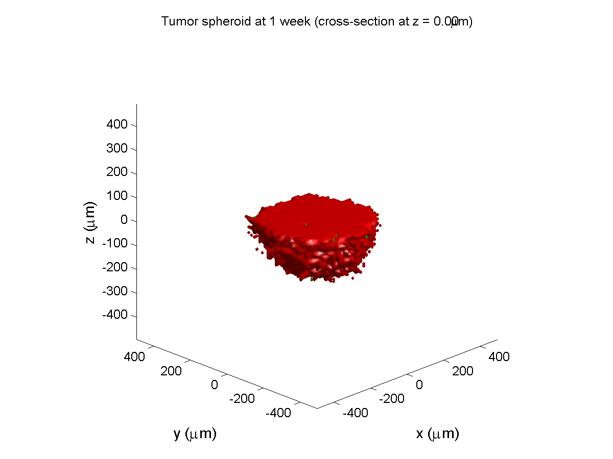
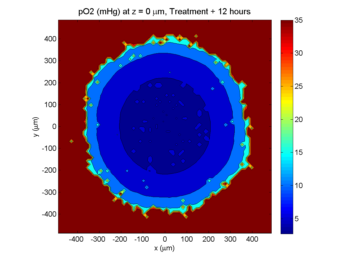
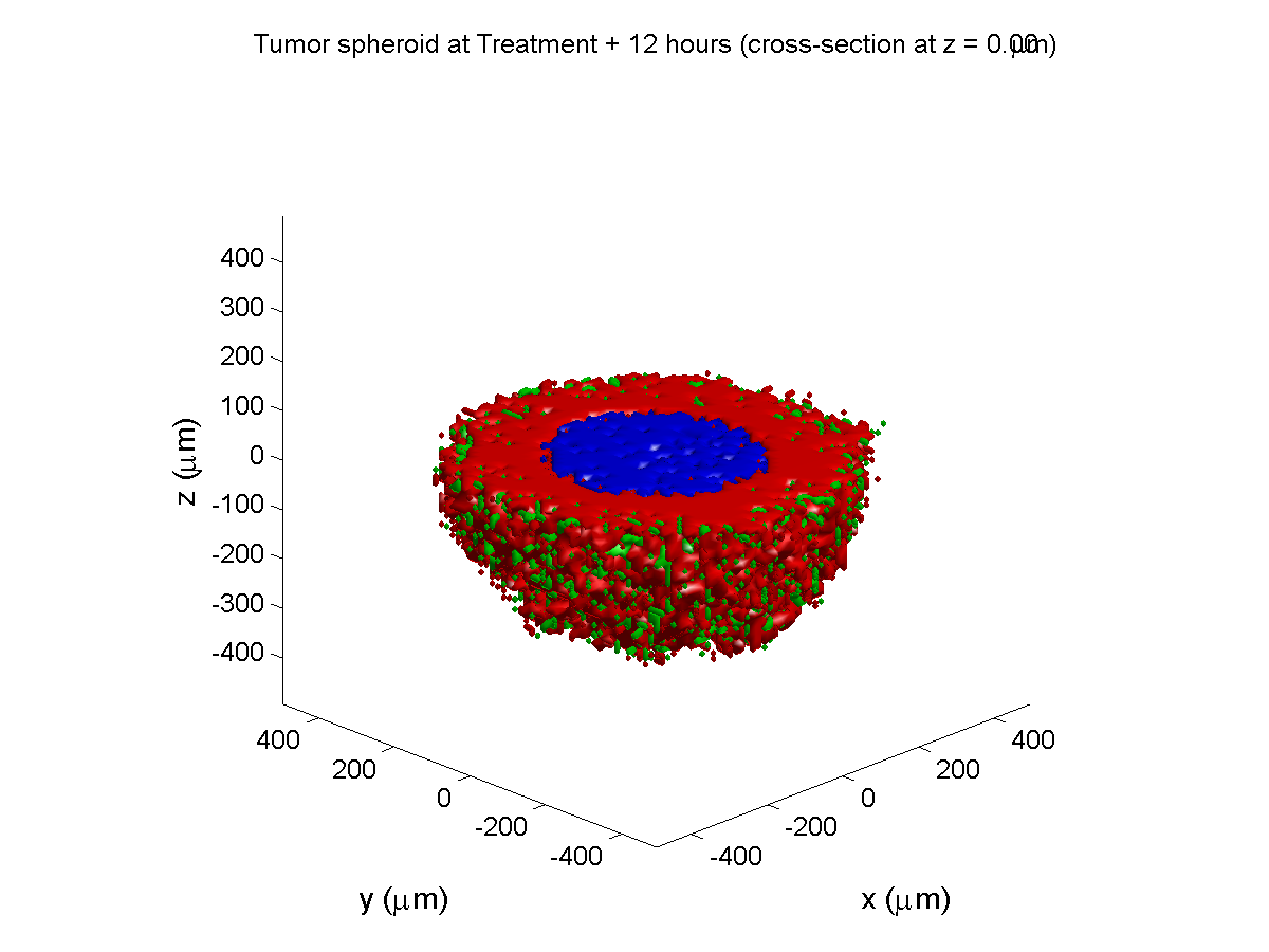
Here are some plots, showing (left from right) pO2 concentration, a cross-section of the tumor (red = live cells, green = apoptotic, and blue = necrotic), and the drug concentration (after start of therapy):
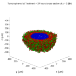
1 week:

Oxygen- and space-limited growth are restricted to the outer boundary of the tumor spheroid.
2 weeks:
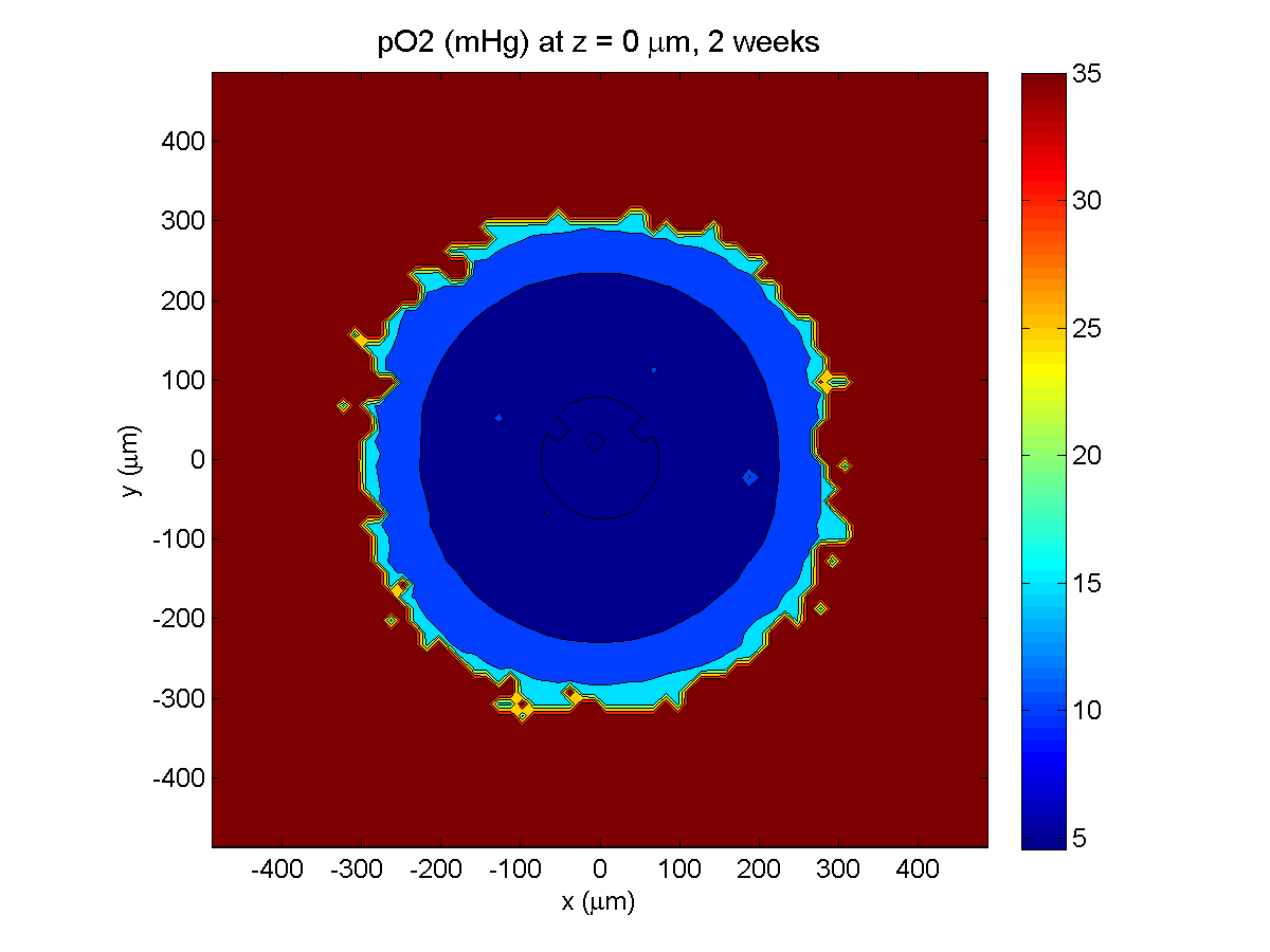
Oxygenation is dipped below 5 mmHg in the center, leading to necrosis.
3 weeks:
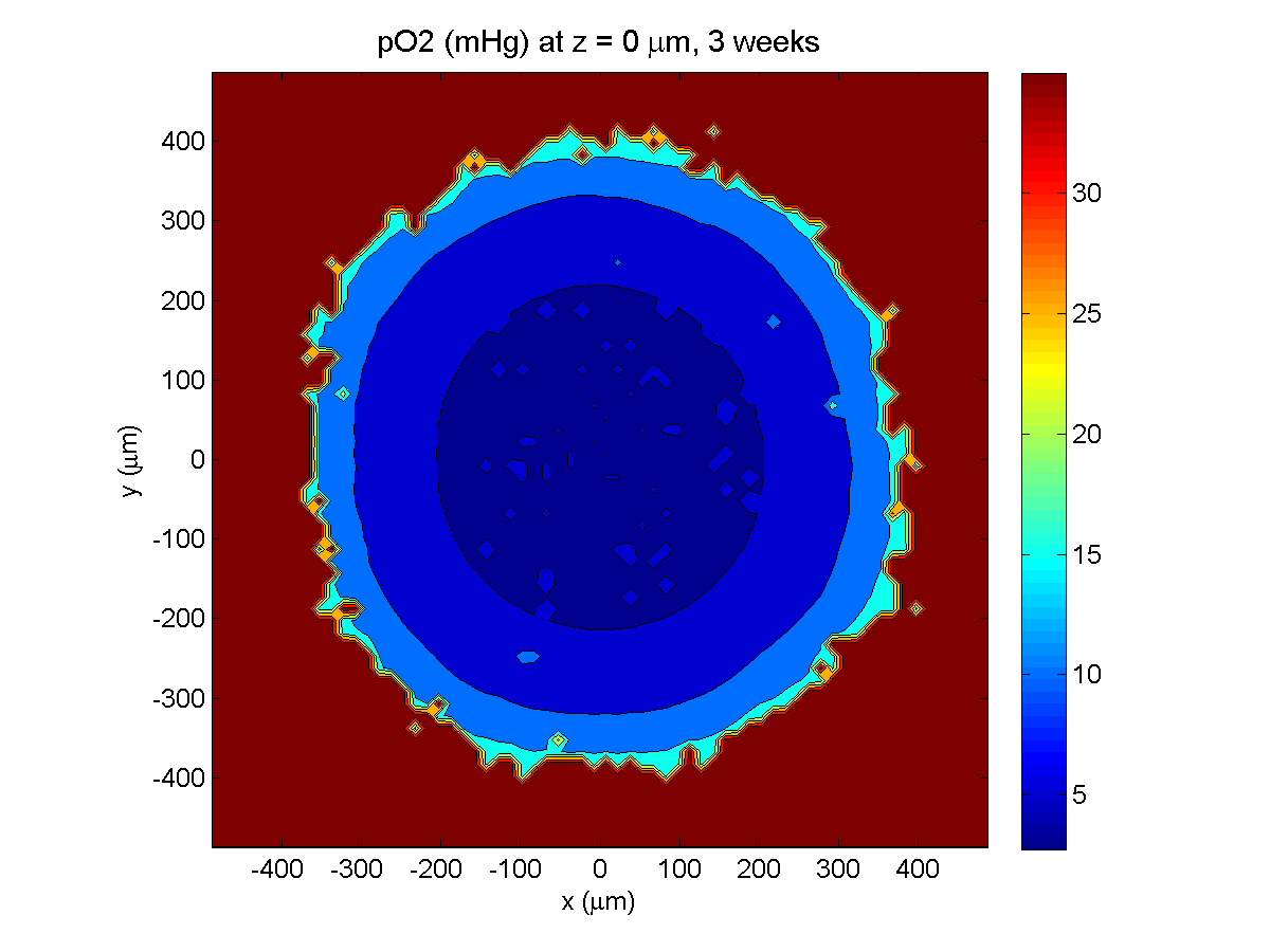
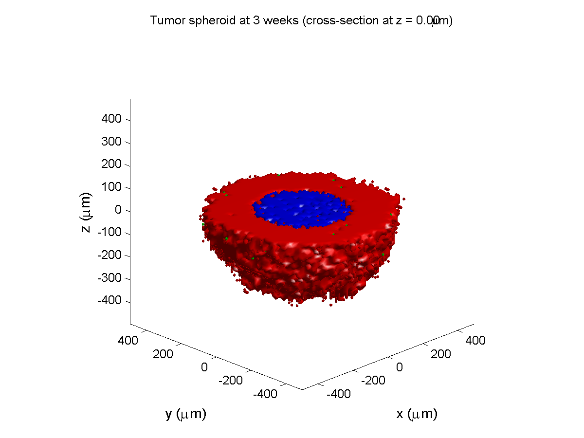
As the tumor grows, the hypoxic gradient increases, and the necrotic core grows. The code turns on a constant 5 micromolar dose of doxorubicin at this point
Treatment + 12 hours:

The drug has started to penetrate the tumor, triggering apoptotic death towards the outer periphery where exposure has been greatest.
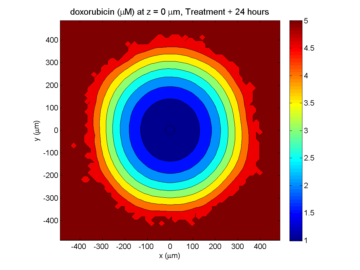
Treatment + 24 hours:


The drug profile hasn’t changed much, but the interior cells have now had greater exposure to drug, and hence greater response. Now apoptosis is observed throughout the non-necrotic tumor. The tumor has decreased in volume somewhat.
Treatment + 36 hours:
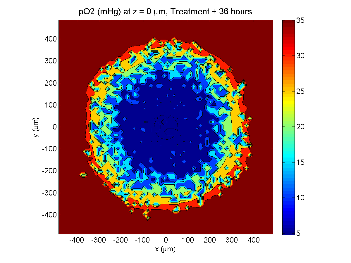
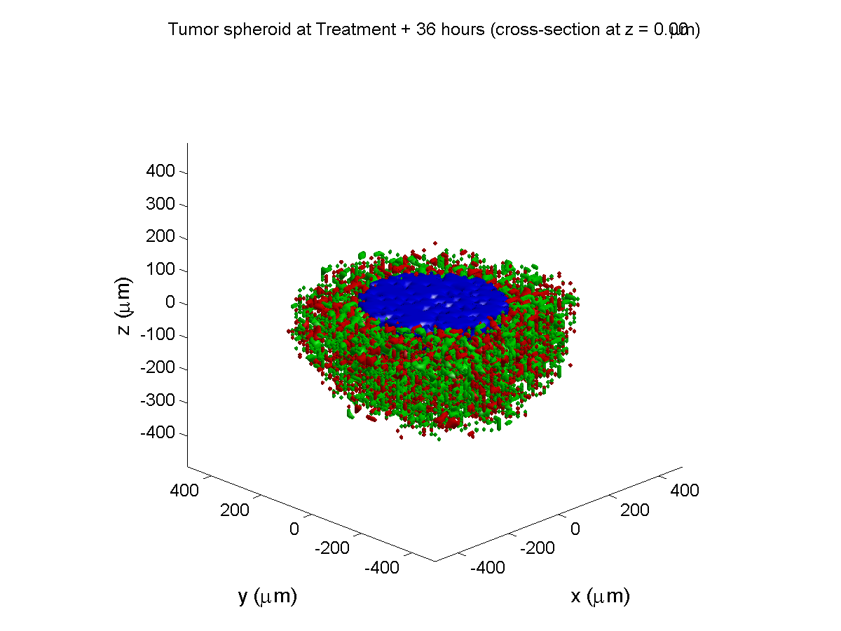
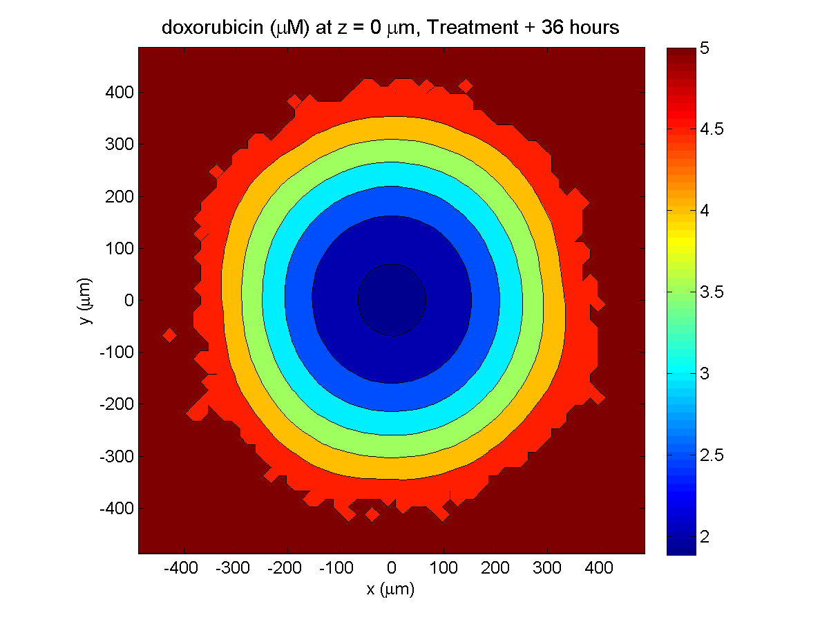
The non-necrotic tumor is now substantially apoptotic. We would require some pharamcokinetic effects (e.g., drug clearance, inactivation, or removal) to avoid the inevitable, presences of a pre-existing resistant strain, or emergence of resistance.
Treatment + 48 hours:
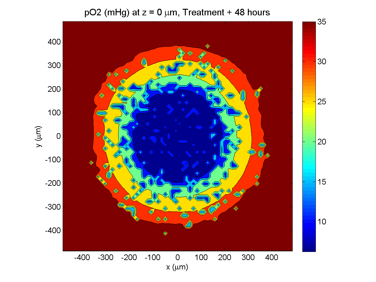
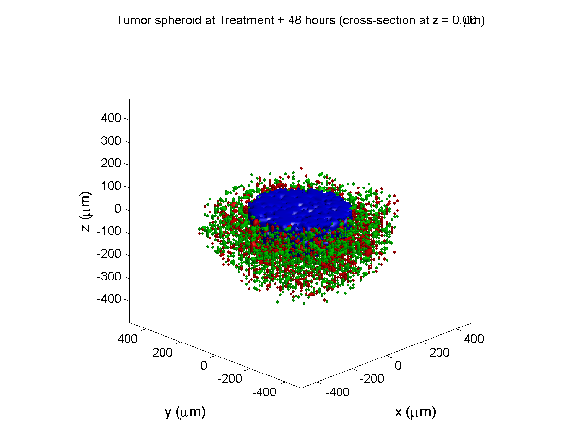
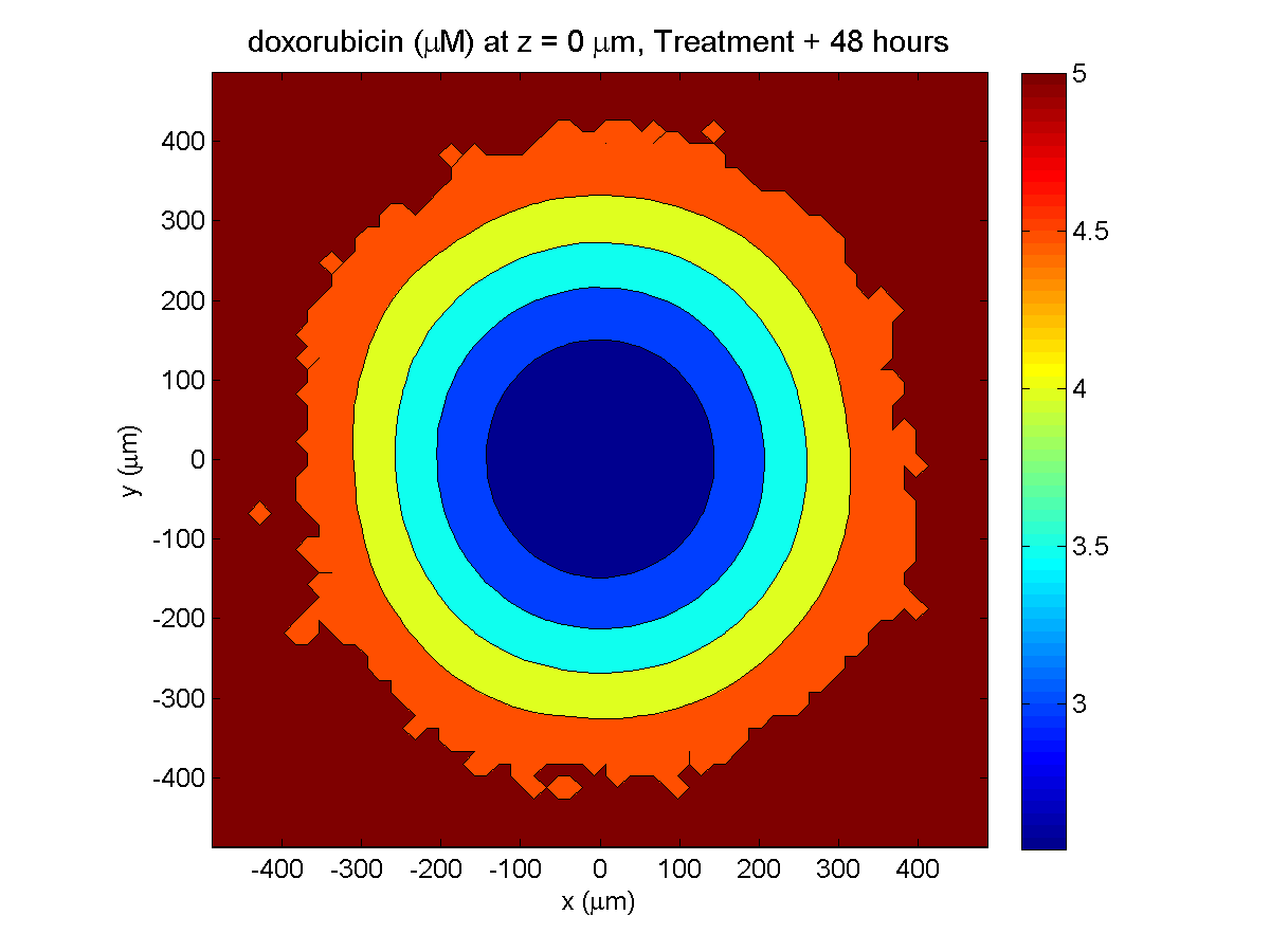
By now, almost all cells are apoptotic.
Treatment + 60 hours:

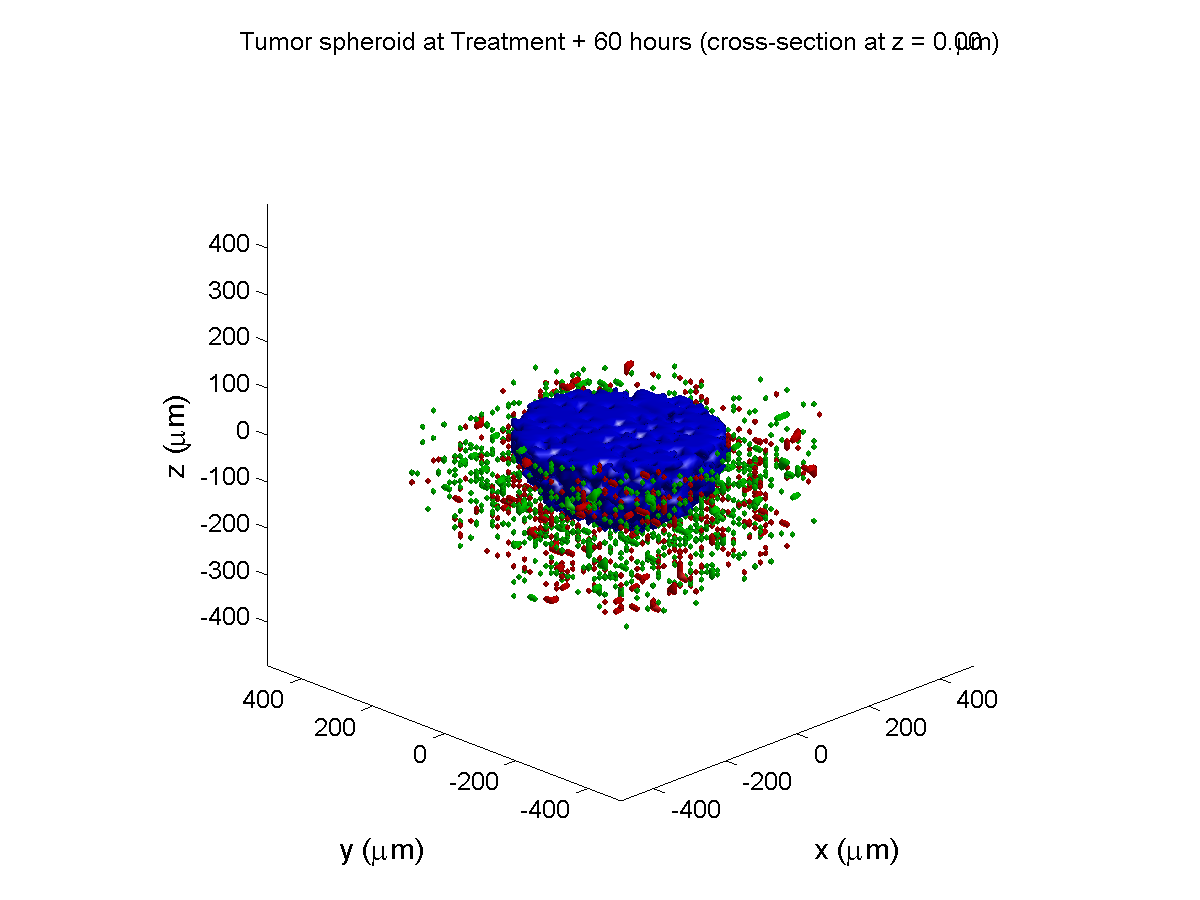

The non-necrotic tumor is nearly completed eliminated, leaving a leftover core of previously-necrotic cells (which did not change state in response to the drug–they were already dead!)
Source files
You can download completed source for this example here: https://sourceforge.net/projects/biofvm/files/Tutorials/Cellular_Automaton_1/
This file will include the following:
- BioFVM_cellular_automata.h
- BioFVM_cellular_automata.cpp
- BioFVM_CA_example_1.cpp
- read_MultiCellDS_xml.m (updated)
- plot_cellular_automata.m
- Makefile
What’s next
I plan to update this source code with extra cell motility, and potentially more realistic parameter values. Also, I plan to more formally separate out the example from the generic cell capabilities, so that this source code can work as a bona fide cellular automaton framework.
More immediately, my next tutorial will use the reverse strategy: start with an existing cellular automaton model, and integrate BioFVM capabilities.
Return to News • Return to MathCancer • Follow @MathCancer