Category: BioFVM
Setting up the PhysiCell microenvironment with XML
As of release 1.6.0, users can define all the chemical substrates in the microenvironment with an XML configuration file. (These are stored by default in ./config/. The default parameter file is ./config/PhysiCell_settings.xml.) This should make it much easier to set up the microenvironment (previously required a lot of manual C++), as well as make it easier to change parameters and initial conditions.
In release 1.7.0, users gained finer grained control on Dirichlet conditions: individual Dirichlet conditions can be enabled or disabled for each individual diffusing substrate on each individual boundary. See details below.
This tutorial will show you the key techniques to use these features. (See the User_Guide for full documentation.) First, let’s create a barebones 2D project by populating the 2D template project. In a terminal shell in your root PhysiCell directory, do this:
make template2D
We will use this 2D project template for the remainder of the tutorial. We assume you already have a working copy of PhysiCell installed, version 1.6.0 or later. (If not, visit the PhysiCell tutorials to find installation instructions for your operating system.) You will need version 1.7.0 or later to control Dirichlet conditions on individual boundaries.
You can download the latest version of PhysiCell at:
- GitHub: https://github.com/MathCancer/PhysiCell/releases
- SourceForge: https://sourceforge.net/projects/physicell/files/latest/download
Microenvironment setup in the XML configuration file
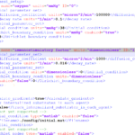
Next, let’s look at the parameter file. In your text editor of choice, open up ./config/PhysiCell_settings.xml, and browse down to <microenvironment_setup>:
<microenvironment_setup>
	<variable name="oxygen" units="mmHg" ID="0">
		<physical_parameter_set>
			<diffusion_coefficient units="micron^2/min">100000.0</diffusion_coefficient>
			<decay_rate units="1/min">0.1</decay_rate>
		</physical_parameter_set>
		<initial_condition units="mmHg">38.0</initial_condition>
		<Dirichlet_boundary_condition units="mmHg" enabled="true">38.0</Dirichlet_boundary_condition>
	</variable>

	<options>
		<calculate_gradients>false</calculate_gradients>
		<track_internalized_substrates_in_each_agent>false</track_internalized_substrates_in_each_agent>
		<!-- not yet supported -->
		<initial_condition type="matlab" enabled="false">
			<filename>./config/initial.mat</filename>
		</initial_condition>
		<!-- not yet supported -->
		<dirichlet_nodes type="matlab" enabled="false">
			<filename>./config/dirichlet.mat</filename>
		</dirichlet_nodes>
	</options>
</microenvironment_setup>
Notice a few trends:
- The <variable> XML element (tag) is used to define a chemical substrate in the microenvironment. The attributes say that it is named oxygen, and the units of measurement are mmHg. Notice also that the ID is 0: this unique integer identifier helps for finding and accessing the substrate within your PhysiCell project. Make sure your first substrate ID is 0, since C++ starts indexing at 0.
- Within the <variable> block, we set the properties of this substrate:
- <diffusion_coefficient> sets the (uniform) diffusion constant for the substrate.
- <decay_rate> is the substrate’s background decay rate.
- <initial_condition> is the value the substrate will be (uniformly) initialized to throughout the domain.
- <Dirichlet_boundary_condition> is the value the substrate will be set to along the outer computational boundary throughout the simulation, if you set enabled=true. If enabled=false, then PhysiCell (via BioFVM) will use Neumann (zero flux) conditions for that substrate.
- The <options> element helps configure other simulation behaviors:
- Use <calculate_gradients> to control whether PhysiCell computes all chemical gradients at each time step. Set this to true to enable accurate gradients (e.g., for chemotaxis).
- Use <track_internalized_substrates_in_each_agent> to enable or disable the PhysiCell feature of actively tracking the total amount of internalized substrates in each individual agent. Set this to true to enable the feature.
- <initial_condition> is reserved for a future release where we can specify non-uniform initial conditions as an external file (e.g., a CSV or Matlab file). This is not yet supported.
- <dirichlet_nodes> is reserved for a future release where we can specify Dirchlet nodes at any location in the simulation domain with an external file. This will be useful for irregular domains, but it is not yet implemented.
Note that PhysiCell does not convert units. The units attributes are helpful for clarity between users and developers, to ensure that you have worked in consistent length and time units. By default, PhysiCell uses minutes for all time units, and microns for all spatial units.
Changing an existing substrate
Let’s modify the oxygen variable to do the following:
- Change the diffusion coefficient to 120000 \(\mu\mathrm{m}^2 / \mathrm{min}\)
- Change the initial condition to 40 mmHg
- Change the oxygen Dirichlet boundary condition to 42.7 mmHg
- Enable gradient calculations
If you modify the appropriate fields in the <microenvironment_setup> block, it should look like this:
<microenvironment_setup>
	<variable name="oxygen" units="mmHg" ID="0">
		<physical_parameter_set>
			<diffusion_coefficient units="micron^2/min">120000.0</diffusion_coefficient>
			<decay_rate units="1/min">0.1</decay_rate>
		</physical_parameter_set>
		<initial_condition units="mmHg">40.0</initial_condition>
		<Dirichlet_boundary_condition units="mmHg" enabled="true">42.7</Dirichlet_boundary_condition>
	</variable>

	<options>
		<calculate_gradients>true</calculate_gradients>
		<track_internalized_substrates_in_each_agent>false</track_internalized_substrates_in_each_agent>
		<!-- not yet supported -->
		<initial_condition type="matlab" enabled="false">
			<filename>./config/initial.mat</filename>
		</initial_condition>
		<!-- not yet supported -->
		<dirichlet_nodes type="matlab" enabled="false">
			<filename>./config/dirichlet.mat</filename>
		</dirichlet_nodes>
	</options>
</microenvironment_setup>
Adding a new diffusing substrate
Let’s add a new dimensionless substrate glucose with the following:
- Diffusion coefficient is 18000 \(\mu\mathrm{m}^2 / \mathrm{min}\)
- No decay rate
- The initial condition is 1 (dimensionless)
- Neumann (no flux) boundary conditions
To add the new variable, I suggest copying an existing variable (in this case, oxygen) and modifying to:
- change the name and units throughout
- increase the ID by one
- write in the appropriate initial and boundary conditions
If you modify the appropriate fields in the <microenvironment_setup> block, it should look like this:
<microenvironment_setup>
	<variable name="oxygen" units="mmHg" ID="0">
		<physical_parameter_set>
			<diffusion_coefficient units="micron^2/min">120000.0</diffusion_coefficient>
			<decay_rate units="1/min">0.1</decay_rate>
		</physical_parameter_set>
		<initial_condition units="mmHg">40.0</initial_condition>
		<Dirichlet_boundary_condition units="mmHg" enabled="true">42.7</Dirichlet_boundary_condition>
	</variable>

	<variable name="glucose" units="dimensionless" ID="1">
		<physical_parameter_set>
			<diffusion_coefficient units="micron^2/min">18000.0</diffusion_coefficient>
			<decay_rate units="1/min">0.0</decay_rate>
		</physical_parameter_set>
		<initial_condition units="dimensionless">1</initial_condition>
		<Dirichlet_boundary_condition units="dimensionless" enabled="false">0</Dirichlet_boundary_condition>
	</variable>

	<options>
		<calculate_gradients>true</calculate_gradients>
		<track_internalized_substrates_in_each_agent>false</track_internalized_substrates_in_each_agent>
		<!-- not yet supported -->
		<initial_condition type="matlab" enabled="false">
			<filename>./config/initial.mat</filename>
		</initial_condition>
		<!-- not yet supported -->
		<dirichlet_nodes type="matlab" enabled="false">
			<filename>./config/dirichlet.mat</filename>
		</dirichlet_nodes>
	</options>
</microenvironment_setup>
Controlling Dirichlet conditions on individual boundaries
In Version 1.7.0, we introduced the ability to control the Dirichlet conditions for each individual boundary for each substrate. The examples above apply (enable) or disable the same condition on each boundary with the same boundary value.
Suppose that we want to set glucose so that the Dirichlet condition is enabled on the bottom z boundary (with value 1) and the left and right x boundaries (with value 0.5) and disabled on all other boundaries. We modify the variable block by adding the optional Dirichlet_options block:
<variable name="glucose" units="dimensionless" ID="1">
	<physical_parameter_set>
		<diffusion_coefficient units="micron^2/min">18000.0</diffusion_coefficient>
		<decay_rate units="1/min">0.0</decay_rate>
	</physical_parameter_set>
	<initial_condition units="dimensionless">1</initial_condition>
	<Dirichlet_boundary_condition units="dimensionless" enabled="true">0</Dirichlet_boundary_condition>
	<Dirichlet_options>
		<boundary_value ID="xmin" enabled="true">0.5</boundary_value>
		<boundary_value ID="xmax" enabled="true">0.5</boundary_value>
		<boundary_value ID="ymin" enabled="false">0.5</boundary_value>
		<boundary_value ID="ymin" enabled="false">0.5</boundary_value>
		<boundary_value ID="zmin" enabled="true">1.0</boundary_value>
		<boundary_value ID="zmax" enabled="false">0.5</boundary_value>
	</Dirichlet_options>
</variable>
Notice a few things:
- The Dirichlet_boundary_condition element has its enabled attribute set to true
- The Dirichlet condition is set under any individual boundary with a boundary_value element.
- The ID attribute indicates which boundary is being specified.
- The enabled attribute allows the individual boundary to be enabled (with value given by the element’s value) or disabled (applying a Neumann or no-flux condition for this substrate at this boundary).
- Any individual boundary indicated by a boundary_value element supersedes the value given by Dirichlet_boundary_condition for this boundary.
Closing thoughts and future work
In the future, we plan to develop more of the options to allow users to set set the initial conditions externally and import them (via an external file), and to allow them to set up more complex domains by importing Dirichlet nodes.
More broadly, we are working to push more model specification from raw C++ to imported XML. It is our hope that this will vastly simplify model development, facilitate creation of graphical model editing tools, and ultimately broaden the class of developers who can use and contribute to PhysiCell. Thanks for giving it a try!
Adding a directory to your Windows path
When you’re setting your BioFVM / PhysiCell g++ development environment, you’ll need to add the compiler, MSYS, and your text editor (like Notepad++) to your system path. For example, you may need to add folders like these to your system PATH variable:
- c:\Program Files\mingw-w64\x86_64-5.3.0-win32-seh-rt_v4_rev0\mingw64\bin\
- c:\Program Files (x86)\Notepad++\
- C:\MinGW\msys\1.0\bin\
Here’s how to do that in various versions of Windows.
Windows XP, 7, and 8
First, open up a text editor, and concatenate your three paths into a single block of text, separated by semicolons (;):
- Open notepad ([Windows]+R, notepad)
- Type a semicolon, paste in the first path, and append a semicolon. It should look like this:
;c:\Program Files\mingw-w64\x86_64-5.3.0-win32-seh-rt_v4_rev0\mingw64\bin\;
- Paste in the next path, and append a semicolon. It should look like this:
;c:\Program Files\mingw-w64\x86_64-5.3.0-win32-seh-rt_v4_rev0\mingw64\bin\;C:\Program Files (x86)\Notepad++\;
- Paste in the last path, and append a semicolon. It should look something like this:
;c:\Program Files\mingw-w64\x86_64-5.3.0-win32-seh-rt_v4_rev0\mingw64\bin\;C:\Program Files (x86)\Notepad++\;c:\MinGW\msys\1.0\bin\;
Lastly, add these paths to the system path:
- Go the Start Menu, the right-click “This PC” or “My Computer”, and choose “Properties.”
- Click on “Advanced system settings”
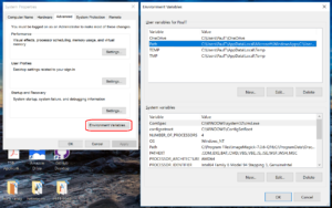
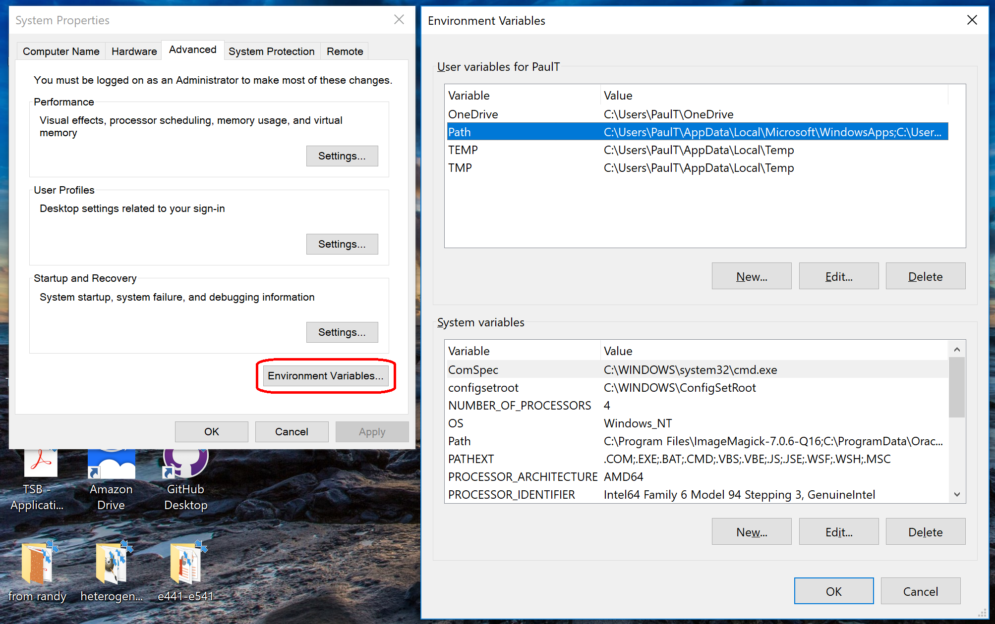
- Click on “Environment Variables…” in the “Advanced” tab
- Scroll through the “System Variables” below until you find Path.
- Select “Path”, then click “Edit…”
- At the very end of “Variable Value”, paste what you made in Notepad in the prior steps. Make sure to paste at the end of the existing value, rather than overwriting it!
- Hit OK, OK, and OK to completely exit the “Advanced system settings.”
Windows 10:
Windows 10 has made it harder to find these settings, but easier to edit them. First, let’s find the system path:
- At the “run / search / Cortana” box next to the start menu, type “view advanced”, and you should see “view advanced system settings” auto-complete:

- Click to enter the advanced system settings, then choose environment variables … at the bottom of this box, and scroll down the list of user variables to Path
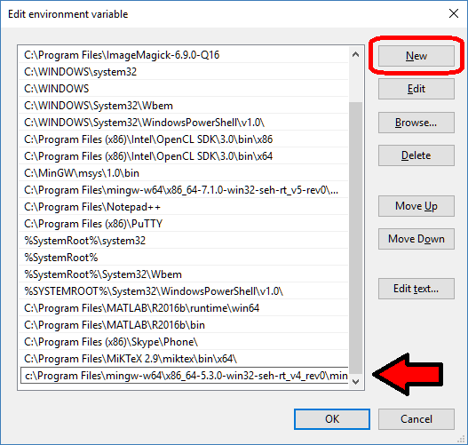
- Click on edit, then click New to add a new path. In the new entry (a new line), paste in your first new path (the compiler):

- Repeat this for the other two paths, then click OK, OK, Apply, OK to apply the new paths and exit.

Working with PhysiCell MultiCellDS digital snapshots in Matlab

PhysiCell 1.2.1 and later saves data as a specialized MultiCellDS digital snapshot, which includes chemical substrate fields, mesh information, and a readout of the cells and their phenotypes at single simulation time point. This tutorial will help you learn to use the matlab processing files included with PhysiCell.
This tutorial assumes you know (1) how to work at the shell / command line of your operating system, and (2) basic plotting and other functions in Matlab.
Key elements of a PhysiCell digital snapshot
A PhysiCell digital snapshot (a customized form of the MultiCellDS digital simulation snapshot) includes the following elements saved as XML and MAT files:
- output12345678.xml : This is the “base” output file, in MultiCellDS format. It includes key metadata such as when the file was created, the software, microenvironment information, and custom data saved at the simulation time. The Matlab files read this base file to find other related files (listed next). Example: output00003696.xml
- initial_mesh0.mat : This is the computational mesh information for BioFVM at time 0.0. Because BioFVM and PhysiCell do not use moving meshes, we do not save this data at any subsequent time.
- output12345678_microenvironment0.mat : This saves each biochemical substrate in the microenvironment at the computational voxels defined in the mesh (see above). Example: output00003696_microenvironment0.mat
- output12345678_cells.mat : This saves very basic cellular information related to BioFVM, including cell positions, volumes, secretion rates, uptake rates, and secretion saturation densities. Example: output00003696_cells.mat
- output12345678_cells_physicell.mat : This saves extra PhysiCell data for each cell agent, including volume information, cell cycle status, motility information, cell death information, basic mechanics, and any user-defined custom data. Example: output00003696_cells_physicell.mat
These snapshots make extensive use of Matlab Level 4 .mat files, for fast, compact, and well-supported saving of array data. Note that even if you cannot ready MultiCellDS XML files, you can work to parse the .mat files themselves.
The PhysiCell Matlab .m files
Every PhysiCell distribution includes some matlab functions to work with PhysiCell digital simulation snapshots, stored in the matlab subdirectory. The main ones are:
- composite_cutaway_plot.m : provides a quick, coarse 3-D cutaway plot of the discrete cells, with different colors for live (red), apoptotic (b), and necrotic (black) cells.
- read_MultiCellDS_xml.m : reads the “base” PhysiCell snapshot and its associated matlab files.
- set_MCDS_constants.m : creates a data structure MCDS_constants that has the same constants as PhysiCell_constants.h. This is useful for identifying cell cycle phases, etc.
- simple_cutaway_plot.m : provides a quick, coarse 3-D cutaway plot of user-specified cells.
- simple_plot.m : provides, a quick, coarse 3-D plot of the user-specified cells, without a cutaway or cross-sectional clipping plane.
A note on GNU Octave
Unfortunately, GNU octave does not include XML file parsing without some significant user tinkering. And one you’re done, it is approximately one order of magnitude slower than Matlab. Octave users can directly import the .mat files described above, but without the helpful metadata in the XML file. We’ll provide more information on the structure of these MAT files in a future blog post. Moreover, we plan to provide python and other tools for users without access to Matlab.
A sample digital snapshot
We provide a 3-D simulation snapshot from the final simulation time of the cancer-immune example in Ghaffarizadeh et al. (2017, in review) at:
The corresponding SVG cross-section for that time (through z = 0 μm) looks like this:
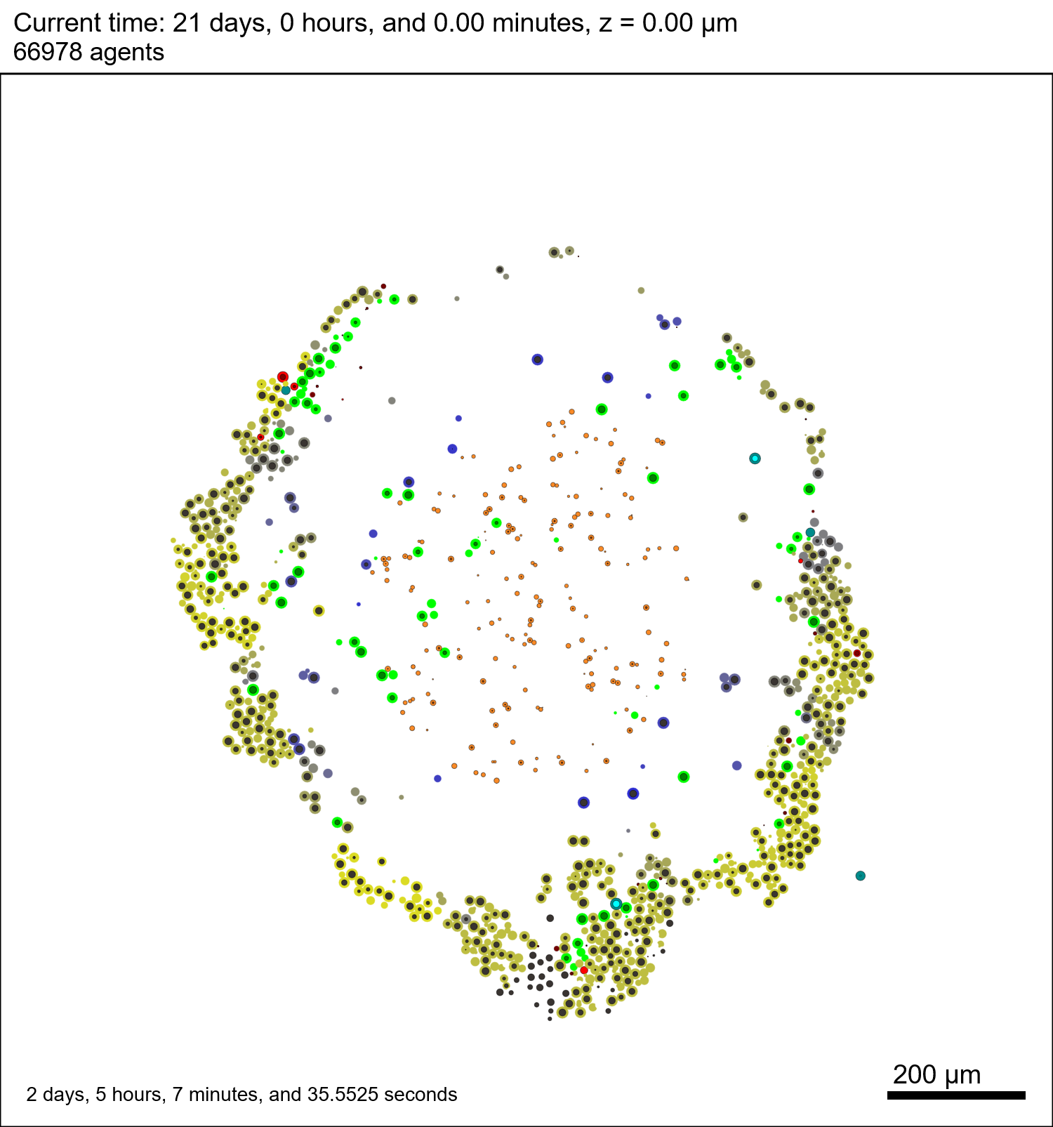
Unzip the sample dataset in any directory, and make sure the matlab files above are in the same directory (or in your Matlab path). If you’re inside matlab:
!unzip 3D_PhysiCell_matlab_sample.zip
Loading a PhysiCell MultiCellDS digital snapshot
Now, load the snapshot:
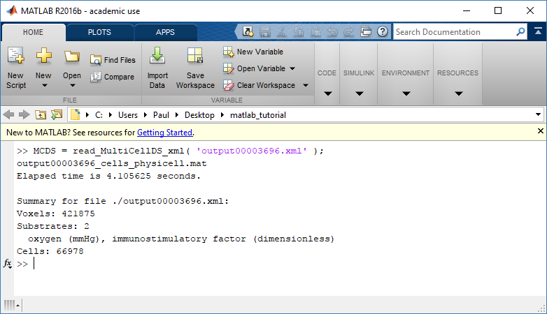
MCDS = read_MultiCellDS_xml( 'output00003696.xml');
This will load the mesh, substrates, and discrete cells into the MCDS data structure, and give a basic summary:
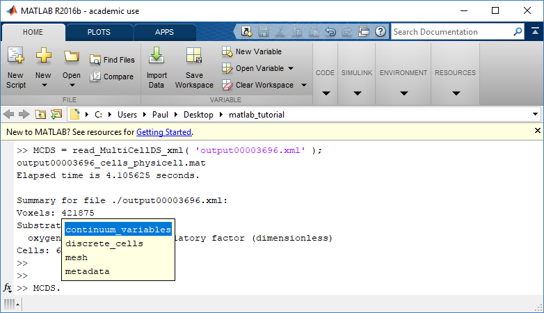
Typing ‘MCDS’ and then hitting ‘tab’ (for auto-completion) shows the overall structure of MCDS, stored as metadata, mesh, continuum variables, and discrete cells:
To get simulation metadata, such as the current simulation time, look at MCDS.metadata.current_time
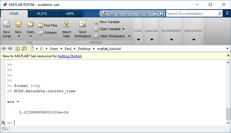
Here, we see that the current simulation time is 30240 minutes, or 21 days. MCDS.metadata.current_runtime gives the elapsed walltime to up to this point: about 53 hours (1.9e5 seconds), including file I/O time to write full simulation data once per 3 simulated minutes after the start of the adaptive immune response.
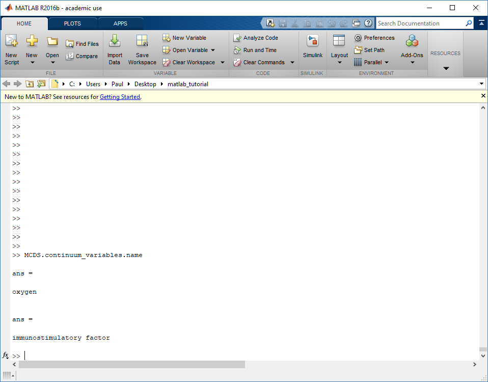
Plotting chemical substrates
Let’s make an oxygen contour plot through z = 0 μm. First, we find the index corresponding to this z-value:
k = find( MCDS.mesh.Z_coordinates == 0 );
Next, let’s figure out which variable is oxygen. Type “MCDS.continuum_variables.name”, which will show the array of variable names:
Here, oxygen is the first variable, (index 1). So, to make a filled contour plot:
contourf( MCDS.mesh.X(:,:,k), MCDS.mesh.Y(:,:,k), ...
     MCDS.continuum_variables(1).data(:,:,k) , 20 ) ;
Now, let’s set this to a correct aspect ratio (no stretching in x or y), add a colorbar, and set the axis labels, using
metadata to get labels:
axis image
colorbar
xlabel( sprintf( 'x (%s)' , MCDS.metadata.spatial_units) );
ylabel( sprintf( 'y (%s)' , MCDS.metadata.spatial_units) );
Lastly, let’s add an appropriate (time-based) title:
title( sprintf('%s (%s) at t = %3.2f %s, z = %3.2f %s', MCDS.continuum_variables(1).name , ...
     MCDS.continuum_variables(1).units , ...
     MCDS.metadata.current_time , ...
     MCDS.metadata.time_units, ...
     MCDS.mesh.Z_coordinates(k), ...
     MCDS.metadata.spatial_units ) );
Here’s the end result:
We can easily export graphics, such as to PNG format:
print( '-dpng' , 'output_o2.png' );
For more on plotting BioFVM data, see the tutorial
at http://www.mathcancer.org/blog/saving-multicellds-data-from-biofvm/
Plotting cells in space
3-D point cloud
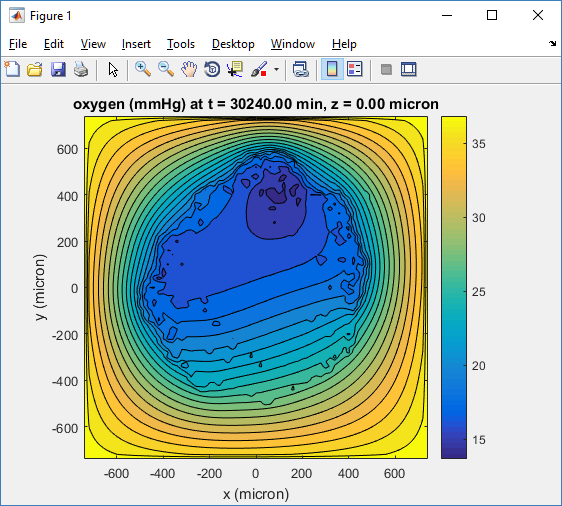
First, let’s plot all the cells in 3D:
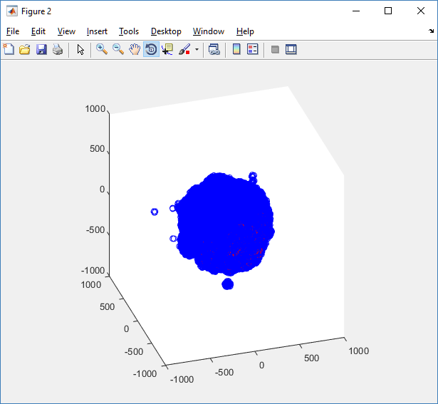
plot3( MCDS.discrete_cells.state.position(:,1) , MCDS.discrete_cells.state.position(:,2), ...
	MCDS.discrete_cells.state.position(:,3) , 'bo' );
At first glance, this does not look good: some cells are far out of the simulation domain, distorting the automatic range of the plot:
This does not ordinarily happen in PhysiCell (the default cell mechanics functions have checks to prevent such behavior), but this example includes a simple Hookean elastic adhesion model for immune cell attachment to tumor cells. In rare circumstances, an attached tumor cell or immune cell can apoptose on its own (due to its background apoptosis rate),
without “knowing” to detach itself from the surviving cell in the pair. The remaining cell attempts to calculate its elastic velocity based upon an invalid cell position (no longer in memory), creating an artificially large velocity that “flings” it out of the simulation domain. Such cells are not simulated any further, so this is effectively equivalent to an extra apoptosis event (only 3 cells are out of the simulation domain after tens of millions of cell-cell elastic adhesion calculations). Future versions of this example will include extra checks to prevent this rare behavior.
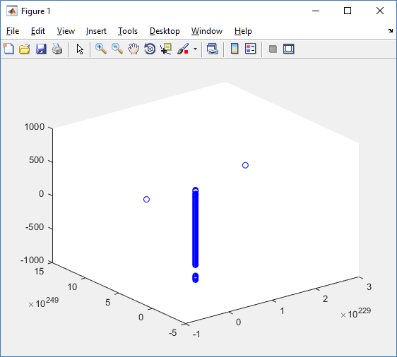
The plot can simply be fixed by changing the axis:
axis( 1000*[-1 1 -1 1 -1 1] )
axis square
Notice that this is a very difficult plot to read, and very non-interactive (laggy) to rotation and scaling operations. We can make a slightly nicer plot by searching for different cell types and plotting them with different colors:
% make it easier to work with the cell positions;
P = MCDS.discrete_cells.state.position;

% find type 1 cells
ind1 = find( MCDS.discrete_cells.metadata.type == 1 );
% better still, eliminate those out of the simulation domain
ind1 = find( MCDS.discrete_cells.metadata.type == 1 & ...
    abs(P(:,1))' < 1000 & abs(P(:,2))' < 1000 & abs(P(:,3))' < 1000 );

% find type 0 cells
ind0 = find( MCDS.discrete_cells.metadata.type == 0 & ...
    abs(P(:,1))' < 1000 & abs(P(:,2))' < 1000 & abs(P(:,3))' < 1000 );

%now plot them
P = MCDS.discrete_cells.state.position;
plot3( P(ind0,1), P(ind0,2), P(ind0,3), 'bo' )
hold on
plot3( P(ind1,1), P(ind1,2), P(ind1,3), 'ro' )
hold off
axis( 1000*[-1 1 -1 1 -1 1] )
axis square
However, this isn’t much better. You can use the scatter3 function to gain more control on the size and color of the plotted cells, or even make macros to plot spheres in the cell locations (with shading and lighting), but Matlab is very slow when plotting beyond 103 cells. Instead, we recommend the faster preview functions below for data exploration, and higher-quality plotting (e.g., by POV-ray) for final publication-
Fast 3-D cell data previewers
Notice that plot3 and scatter3 are painfully slow for any nontrivial number of cells. We can use a few fast previewers to quickly get a sense of the data. First, let’s plot all the dead cells, and make them red:
clf
simple_plot( MCDS,  MCDS, MCDS.discrete_cells.dead_cells , 'r' )
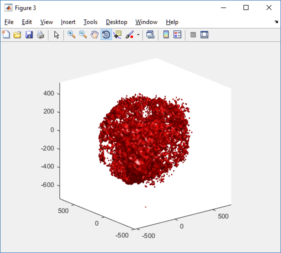
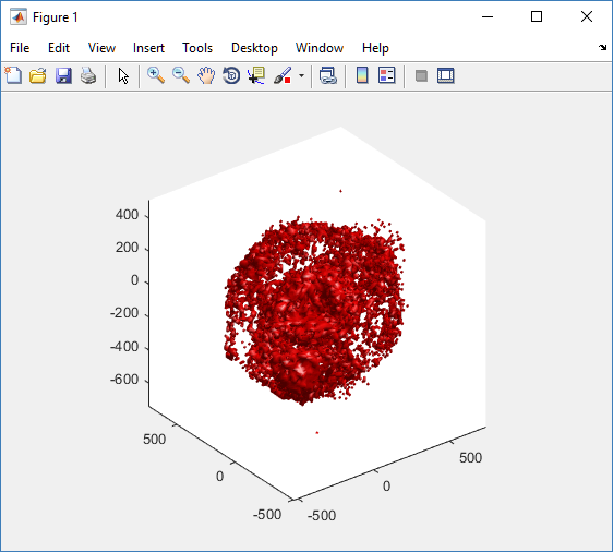
This function creates a coarse-grained 3-D indicator function (0 if no cells are present; 1 if they are), and plots a 3-D level surface. It is very responsive to rotations and other operations to explore the data. You may notice the second argument is a list of indices: only these cells are plotted. This gives you a method to select cells with specific characteristics when plotting. (More on that below.) If you want to get a sense of the interior structure, use a cutaway plot:
clf
simple_cutaway_plot( MCDS, MCDS, MCDS.discrete_cells.dead_cells , 'r' )
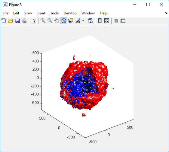
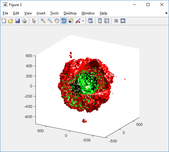
We also provide a fast “composite” cutaway which plots all live cells as red, apoptotic cells as blue (without the cutaway), and all necrotic cells as black:
clf
composite_cutaway_plot( MCDS )
Lastly, we show an improved plot that uses different colors for the immune cells, and Matlab’s “find” function to help set up the indexing:
constants = set_MCDS_constants

% find the type 0 necrotic cells
ind0_necrotic = find( MCDS.discrete_cells.metadata.type == 0 & ...
    (MCDS.discrete_cells.phenotype.cycle.current_phase == constants.necrotic_swelling | ...
    MCDS.discrete_cells.phenotype.cycle.current_phase == constants.necrotic_lysed | ...
    MCDS.discrete_cells.phenotype.cycle.current_phase == constants.necrotic) );

% find the live type 0 cells
ind0_live = find( MCDS.discrete_cells.metadata.type == 0 & ...
    (MCDS.discrete_cells.phenotype.cycle.current_phase ~= constants.necrotic_swelling & ...
    MCDS.discrete_cells.phenotype.cycle.current_phase ~= constants.necrotic_lysed & ...
    MCDS.discrete_cells.phenotype.cycle.current_phase ~= constants.necrotic & ...
    MCDS.discrete_cells.phenotype.cycle.current_phase ~= constants.apoptotic) );

clf
% plot live tumor cells red, in cutaway view
simple_cutaway_plot( MCDS, ind0_live , 'r' );
hold on
% plot dead tumor cells black, in cutaway view
simple_cutaway_plot( MCDS, ind0_necrotic , 'k' )
% plot all immune cells, but without cutaway (to show how they infiltrate)
simple_plot( MCDS, ind1, 'g' )
hold off
A small cautionary note on future compatibility
PhysiCell 1.2.1 uses the <custom> data tag (allowed as part of the MultiCellDS specification) to encode its cell data, to allow a more compact data representation, because the current PhysiCell daft does not support such a formulation, and Matlab is painfully slow at parsing XML files larger than ~50 MB. Thus, PhysiCell snapshots are not yet fully compatible with general MultiCellDS tools, which would by default ignore custom data. In the future, we will make available converter utilities to transform “native” custom PhysiCell snapshots to MultiCellDS snapshots that encode all the cellular information in a more verbose but compatible XML format.
Closing words and future work
Because Octave is not a great option for parsing XML files (with critical MultiCellDS metadata), we plan to write similar functions to read and plot PhysiCell snapshots in Python, as an open source alternative. Moreover, our lab in the next year will focus on creating further MultiCellDS configuration, analysis, and visualization routines. We also plan to provide additional 3-D functions for plotting the discrete cells and varying color with their properties.
In the longer term, we will develop open source, stand-alone analysis and visualization tools for MultiCellDS snapshots (including PhysiCell snapshots). Please stay tuned!
Getting started with a PhysiCell Virtual Appliance
Note: This is part of a series of “how-to” blog posts to help new users and developers of BioFVM and PhysiCell. This guide is for for users in OSX, Linux, or Windows using the VirtualBox virtualization software to run a PhysiCell virtual appliance.
These instructions should get you up and running without needed to install a compiler, makefile capabilities, or any other software (beyond the virtual machine and the PhysiCell virtual appliance). We note that using the PhysiCell source with your own compiler is still the preferred / ideal way to get started, but the virtual appliance option is a fast way to start even if you’re having troubles setting up your development environment.
What’s a Virtual Machine? What’s a Virtual Appliance?
A virtual machine is a full simulated computer (with its own disk space, operating system, etc.) running on another. They are designed to let a user test on a completely different environment, without affecting the host (main) environment. They also allow a very robust way of taking and reproducing the state of a full working environment.
A virtual appliance is just this: a full image of an installed system (and often its saved state) on a virtual machine, which can easily be installed on a new virtual machine. In this tutorial, you will download our PhysiCell virtual appliance and use its pre-configured compiler and other tools.
What you’ll need:
- VirtualBox: This is a free, cross-platform program to run virtual machines on OSX, Linux, Windows, and other platforms. It is a safe and easy way to install one full operating (a client system) on your main operating system (the host system). For us, this means that we can distribute a fully working Linux environment with a working copy of all the tools you need to compile and run PhysiCell. As of August 1, 2017, this will download Version 5.1.26.
- Download here: https://www.virtualbox.org/wiki/Downloads
- PhysiCell Virtual Appliance: This is a single-file distribution of a virtual machine running Alpine Linux, including all key tools needed to compile and run PhysiCell. As of July 31, 2017, this will download PhysiCell 1.2.2 with g++ 6.3.0.
- Download here: https://sourceforge.net/projects/physicell/files/PhysiCell/
- (Browse to a version of PhysiCell, and download the file that ends in “.ova”.)
- Version 1.2.0: http://bit.ly/2vY51P1 [sf.net]
- Download here: https://sourceforge.net/projects/physicell/files/PhysiCell/
- A computer with hardware support for virtualization: Your CPU needs to have hardware support for virtualization (almost all of them do now), and it has to be enabled in your BIOS. Consult your computer maker on how to turn this on if you get error messages later.
Main steps:
1) Install VirtualBox.
Double-click / open the VirtualBox download. Go ahead and accept all the default choices. If asked, go ahead and download/install the extensions pack.
2) Import the PhysiCell Virtual Appliance
Go the “File” menu and choose “Import Virtual Appliance”. Browse to find the .ova file you just downloaded.
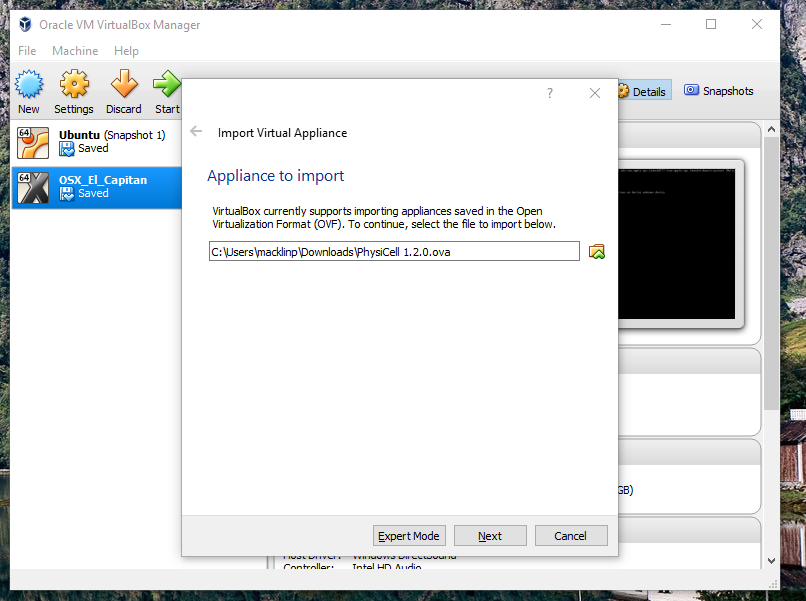
Click on “Next,” and import with all the default options. That’s it!
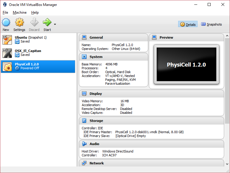
3) [Optional] Change settings
You most likely won’t need this step, but you can increase/decrease the amount of RAM used for the virtual machine if you select the PhysiCell VM, click the Settings button (orange gear), and choose “System”: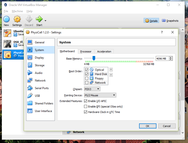 We set the Virtual Machine to have 4 GB of RAM. If you have a machine with lots of RAM (16 GB or more), you may want to set this to 8 GB.
Also, you can choose how many virtual CPUs to give to your VM: 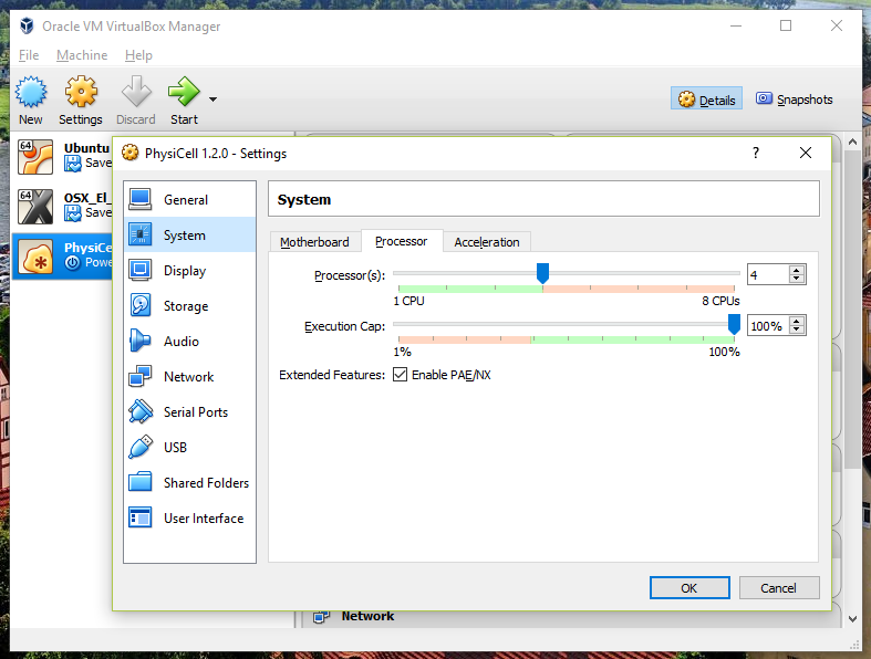
We selected 4 when we set up the Virtual Appliance, but you should match the number of physical processor cores on your machine. In my case, I have a quad core processor with hyperthreading. This means 4 real cores, 8 virtual cores, so I select 4 here.
4) Start the Virtual Machine and log in
Select the PhysiCell machine, and click the green “start” button. After the virtual machine boots (with the good old LILO boot manager that I’ve missed), you should see this: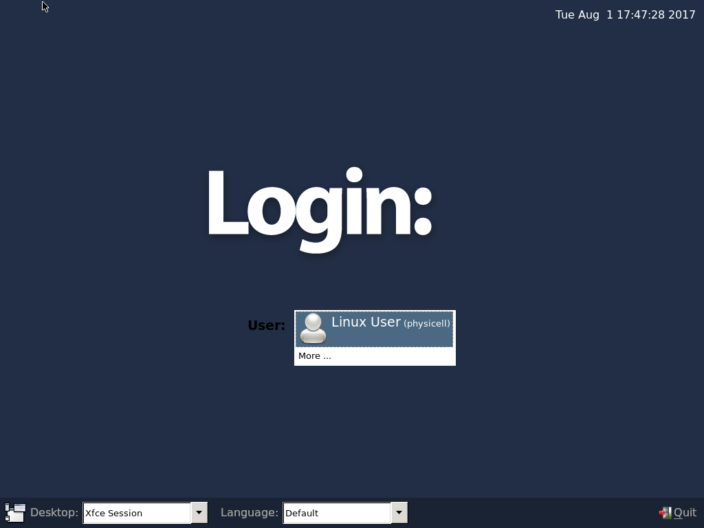
Click the "More ..." button, and log in with username: physicell, password: physicell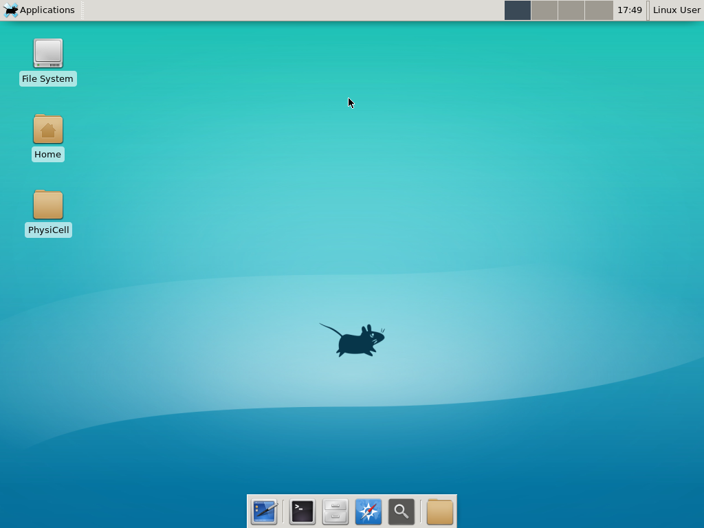
5) Test the compiler and run your first simulation
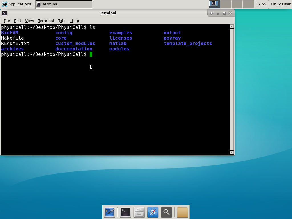
Notice that PhysiCell is already there on the desktop in the PhysiCell folder. Right-click, and choose “open terminal here.” You’ll already be in the main PhysiCell root directory. 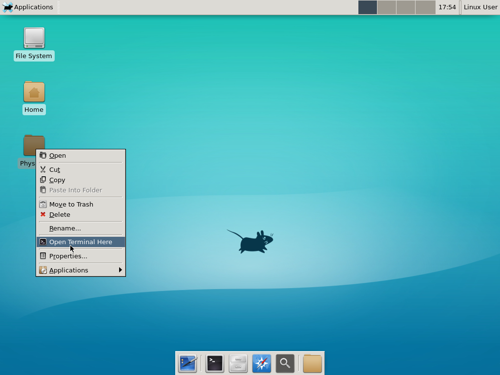
Now, let’s compile your first project! Type “make template2D && make” 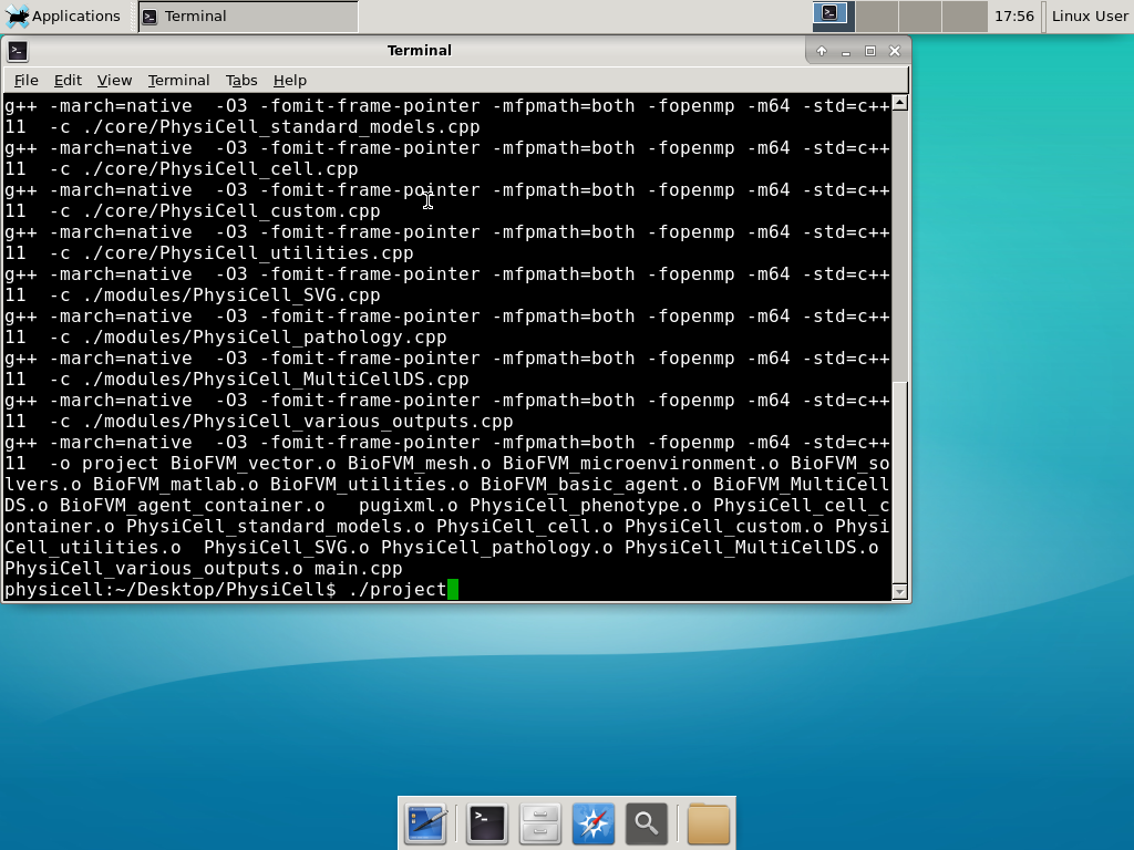 And run your project! Type “./project” and let it go!
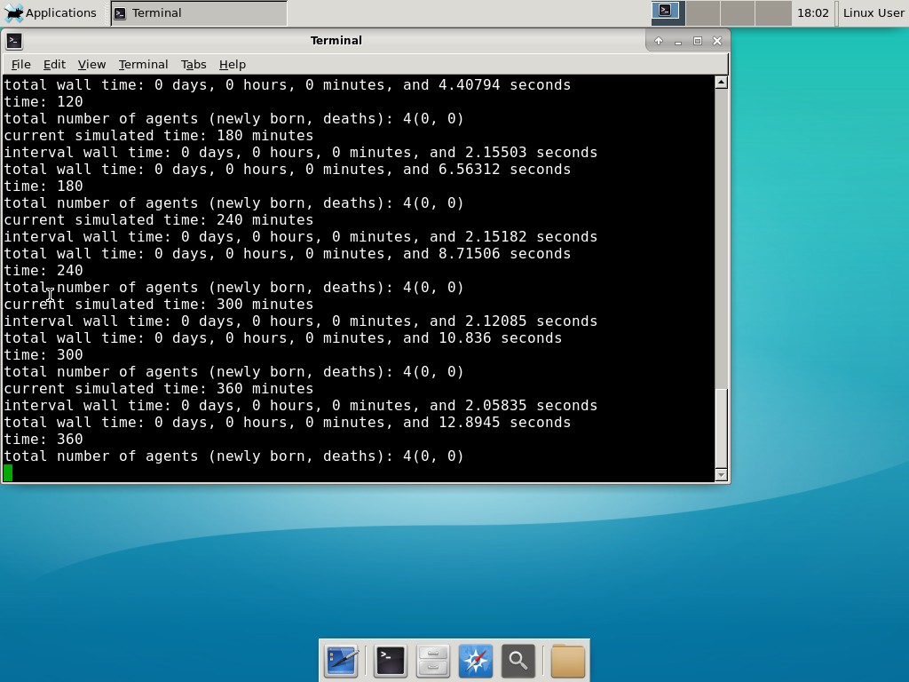 Go ahead and run either the first few days of the simulation (until about 7200 minutes), then hit <control>-C to cancel out. Or run the whole simulation–that’s fine, too.
6) Look at the results
We bundled a few tools to easily look at results. First, ristretto is a very fast image viewer. Let’s view the SVG files: 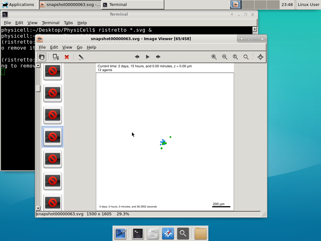 As a nice tip, you can press the left and right arrows to advance through the SVG images, or hold the right arrow down to advance through quickly.
Now, let’s use ImageMagick to convert the SVG files into JPG file: call “magick mogrify -format jpg snap*.svg”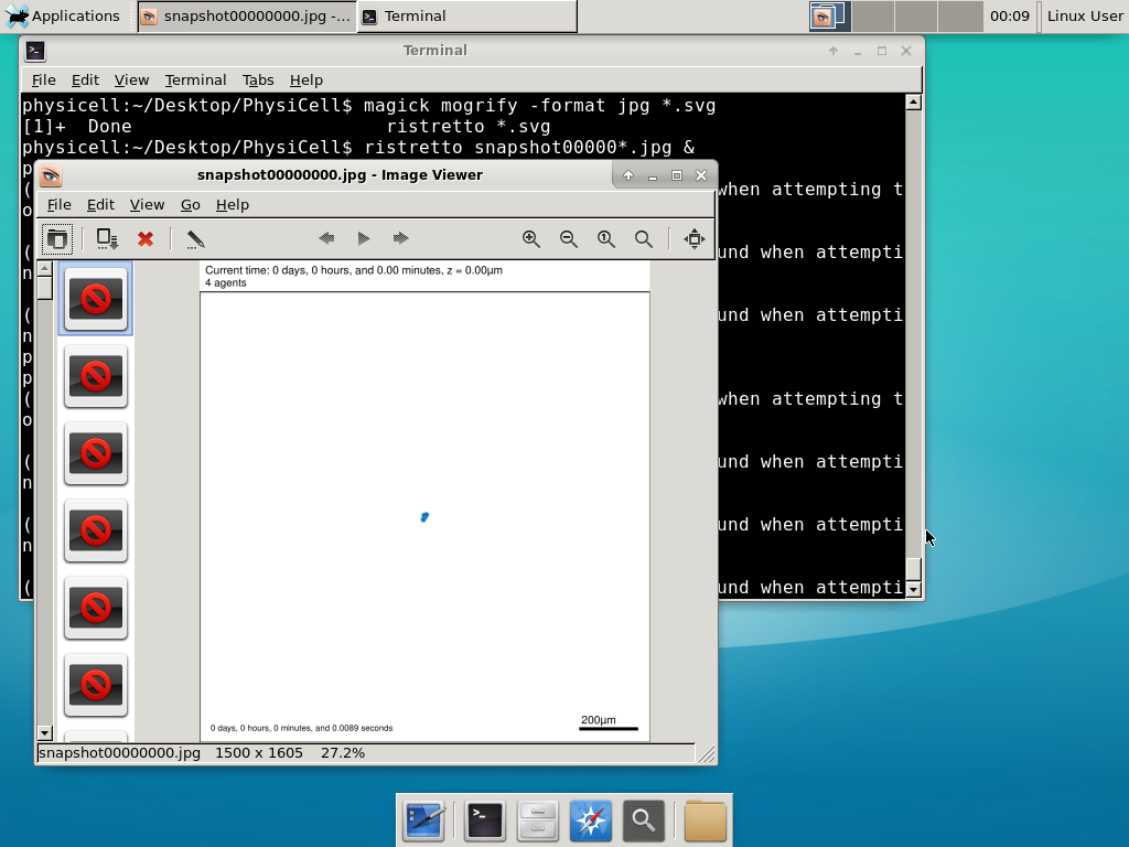
Next, let’s turn those images into a movie. I generally create moves that are 24 frames pers se, so that 1 second of the movie is 1 hour of simulations time. We’ll use mencoder, with options below given to help get a good quality vs. size tradeoff: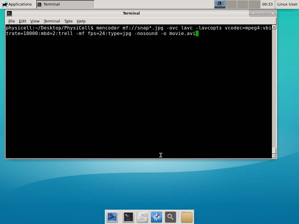
When you’re done, view the movie with mplayer. The options below scale the window to fit within the virtual monitor:
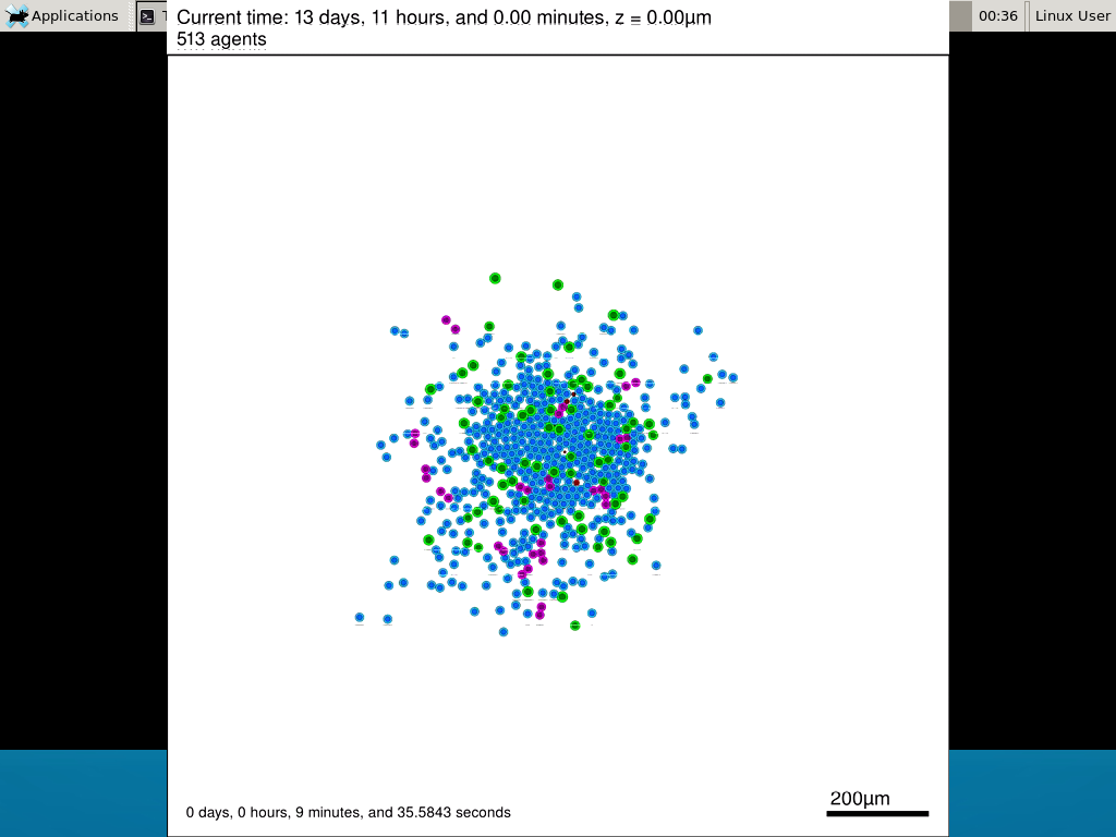
If you want to loop the movie, add “-loop 999” to your command.
7) Get familiar with other tools
Use nano (useage: nano <filename>) to quickly change files at the command line. Hit <control>-O to save your results. Hit <control>-X to exit. <control>-W will search within the file.
Use nedit (useage: nedit <filename> &) to open up one more text files in a graphical editor. This is a good way to edit multiple files at once.
Sometimes, you need to run commands at elevated (admin or root) privileges. Use sudo. Here’s an example, searching the Alpine Linux package manager apk for clang:
physicell:~$ sudo apk search gcc
[sudo] password for physicell:
physicell:~$ sudo apk search clang
clang-analyzer-4.0.0-r0
clang-libs-4.0.0-r0
clang-dev-4.0.0-r0
clang-static-4.0.0-r0
emscripten-fastcomp-1.37.10-r0
clang-doc-4.0.0-r0
clang-4.0.0-r0
physicell:~/Desktop/PhysiCell$
If you want to install clang/llvm (as an alternative compiler):
physicell:~$ sudo apk add gcc
[sudo] password for physicell:
physicell:~$ sudo apk search clang
clang-analyzer-4.0.0-r0
clang-libs-4.0.0-r0
clang-dev-4.0.0-r0
clang-static-4.0.0-r0
emscripten-fastcomp-1.37.10-r0
clang-doc-4.0.0-r0
clang-4.0.0-r0
physicell:~/Desktop/PhysiCell$
Notice that it asks for a password: use the password for root (which is physicell).
8) [Optional] Configure a shared folder
Coming soon.
Why both with zipped source, then?
Given that we can get a whole development environment by just downloading and importing a virtual appliance, why
bother with all the setup of a native development environment, like this tutorial (Windows) or this tutorial (Mac)?
One word: performance. In my testing, I still have not found the performance running inside a
virtual machine to match compiling and running directly on your system. So, the Virtual Appliance is a great
option to get up and running quickly while trying things out, but I still recommend setting up natively with
one of the tutorials I linked in the preceding paragraphs.
What’s next?
In the coming weeks, we’ll post further tutorials on using PhysiCell. In the meantime, have a look at the
PhysiCell project website, and these links as well:
- BioFVM on MathCancer.org: http://BioFVM.MathCancer.org
- BioFVM on SourceForge: http://BioFVM.sf.net
- BioFVM Method Paper in BioInformatics: http://dx.doi.org/10.1093/bioinformatics/btv730
- PhysiCell on MathCancer.org: http://PhysiCell.MathCancer.org
- PhysiCell on Sourceforge: http://PhysiCell.sf.net
- PhysiCell Method Paper (preprint): https://doi.org/10.1101/088773
- PhysiCell tutorials: [click here]
MathCancer C++ Style and Practices Guide
As PhysiCell, BioFVM, and other open source projects start to gain new users and contributors, it’s time to lay out a coding style. We have three goals here:
- Consistency: It’s easier to understand and contribute to the code if it’s written in a consistent way.
- Readability: We want the code to be as readable as possible.
- Reducing errors: We want to avoid coding styles that are more prone to errors. (e.g., code that can be broken by introducing whitespace).
So, here is the guide (revised June 2017). I expect to revise this guide from time to time.
Place braces on separate lines in functions and classes.
I find it much easier to read a class if the braces are on separate lines, with good use of whitespace. Remember: whitespace costs almost nothing, but reading and understanding (and time!) are expensive.
DON’T
class Cell{
public:
 double some_variable;
 bool some_extra_variable;

 Cell(); };

class Phenotype{
public:
 double some_variable;
 bool some_extra_variable;

 Phenotype();
};
DO:
class Cell
{
 public:
     double some_variable;
     bool some_extra_variable;

     Cell();
};

class Phenotype
{
 public:
     double some_variable;
     bool some_extra_variable;

     Phenotype();
};
Enclose all logic in braces, even when optional.
In C/C++, you can omit the curly braces in some cases. For example, this is legal
if( distance > 1.5*cell_radius )
     interaction = false;
force = 0.0; // is this part of the logic, or a separate statement?
error = false;
However, this code is ambiguous to interpret. Moreover, small changes to whitespace–or small additions to the logic–could mess things up here. Use braces to make the logic crystal clear:
DON’T
if( distance > 1.5*cell_radius )
     interaction = false;
force = 0.0; // is this part of the logic, or a separate statement?
error = false;

if( condition1 == true )
  do_something1 = true;
elseif( condition2 == true )
  do_something2 = true;
else
  do_something3 = true;
DO
if( distance > 1.5*cell_radius )
{
     interaction = false;
     force = 0.0;
}
error = false;

if( condition1 == true )
{ do_something1 = true; }
elseif( condition2 == true )
{ do_something2 = true; }
else
{ do_something3 = true; }
Put braces on separate lines in logic, except for single-line logic.
This style rule relates to the previous point, to improve readability.
DON’T
if( distance > 1.5*cell_radius ){
     interaction = false;
     force = 0.0; }

if( condition1 == true ){ do_something1 = true; }
elseif( condition2 == true ){
  do_something2 = true; }
else
{ do_something3 = true; error = true; }
DO
if( distance > 1.5*cell_radius )
{
     interaction = false;
     force = 0.0;
}

if( condition1 == true )
{ do_something1 = true; } // this is fine
elseif( condition2 == true )
{
     do_something2 = true; // this is better
}
else
{
     do_something3 = true;
     error = true;
}
See how much easier that code is to read? The logical structure is crystal clear, and adding more to the logic is simple.
End all functions with a return, even if void.
For clarity, definitively state that a function is done by using return.
DON’T
void my_function( Cell& cell )
{
     cell.phenotype.volume.total *= 2.0;
     cell.phenotype.death.rates[0] = 0.02;
     // Are we done, or did we forget something?
     // is somebody still working here?
}
DO
void my_function( Cell& cell )
{
     cell.phenotype.volume.total *= 2.0;
     cell.phenotype.death.rates[0] = 0.02;
     return;
}
Use tabs to indent the contents of a class or function.
This is to make the code easier to read. (Unfortunately PHP/HTML makes me use five spaces here instead of tabs.)
DON’T
class Secretion
{
 public:
std::vector<double> secretion_rates;
std::vector<double> uptake_rates;
std::vector<double> saturation_densities;
};

void my_function( Cell& cell )
{
cell.phenotype.volume.total *= 2.0;
cell.phenotype.death.rates[0] = 0.02;
return;
}
DO
class Secretion
{
 public:
     std::vector<double> secretion_rates;
     std::vector<double> uptake_rates;
     std::vector<double> saturation_densities;
};

void my_function( Cell& cell )
{
     cell.phenotype.volume.total *= 2.0;
     cell.phenotype.death.rates[0] = 0.02;
     return;
}
Use a single space to indent public and other keywords in a class.
This gets us some nice formatting in classes, without needing two tabs everywhere.
DON’T
class Secretion
{
public:
std::vector<double> secretion_rates;
std::vector<double> uptake_rates;
std::vector<double> saturation_densities;
}; // not enough whitespace

class Errors
{
     private:
          std::string none_of_your_business
     public:
          std::string error_message;
          int error_code;
}; // too much whitespace!
DO
class Secretion
{
 private:
 public:
     std::vector<double> secretion_rates;
     std::vector<double> uptake_rates;
     std::vector<double> saturation_densities;
};

class Errors
{
 private:
     std::string none_of_your_business
 public:
     std::string error_message;
     int error_code;
};
Avoid arcane operators, when clear logic statements will do.
It can be difficult to decipher code with statements like this:
phenotype.volume.fluid=phenotype.volume.fluid<0?0:phenotype.volume.fluid;
Moreover, C and C++ can treat precedence of ternary operators very differently, so subtle bugs can creep in when using the “fancier” compact operators. Variations in how these operators work across languages are an additional source of error for programmers switching between languages in their daily scientific workflows. Wherever possible (and unless there is a significant performance reason to do so), use clear logical structures that are easy to read even if you only dabble in C/C++. Compiler-time optimizations will most likely eliminate any performance gains from these goofy operators.
DON’T
// if the fluid volume is negative, set it to zero
phenotype.volume.fluid=phenotype.volume.fluid<0.0?0.0:pCell->phenotype.volume.fluid;
DO
if( phenotype.volume.fluid < 0.0 )
{
     phenotype.volume.fluid = 0.0;
}
Here’s the funny thing: the second logic is much clearer, and it took fewer characters, even with extra whitespace for readability!
Pass by reference where possible.
Passing by reference is a great way to boost performance: we can avoid (1) allocating new temporary memory, (2) copying data into the temporary memory, (3) passing the temporary data to the function, and (4) deallocating the temporary memory once finished.
DON’T
double some_function( Cell cell )
{
     return = cell.phenotype.volume.total + 3.0;
}
// This copies cell and all its member data!
DO
double some_function( Cell& cell )
{
     return = cell.phenotype.volume.total + 3.0;
}
// This just accesses the original cell data without recopying it.
Where possible, pass by reference instead of by pointer.
There is no performance advantage to passing by pointers over passing by reference, but the code is simpler / clearer when you can pass by reference. It makes code easier to write and understand if you can do so. (If nothing else, you save yourself character of typing each time you can replace “->” by “.”!)
DON’T
double some_function( Cell* pCell )
{
     return = pCell->phenotype.volume.total + 3.0;
}
// Writing and debugging this code can be error-prone.
DO
double some_function( Cell& cell )
{
     return = cell.phenotype.volume.total + 3.0;
}
// This is much easier to write.
Be careful with static variables. Be thread safe!
PhysiCell relies heavily on parallelization by OpenMP, and so you should write functions under the assumption that they may be executed many times simultaneously. One easy source of errors is in static variables:
DON’T
double some_function( Cell& cell )
{
     static double four_pi = 12.566370614359172;
     static double output;
     output = cell.phenotype.geometry.radius;
     output *= output;
     output *= four_pi;
     return output;
}
// If two instances of some_function are running, they will both modify
// the *same copy* of output
DO
double some_function( Cell& cell )
{
     static double four_pi = 12.566370614359172;
     double output;
     output = cell.phenotype.geometry.radius;
     output *= output;
     output *= four_pi;
     return output;
}
// If two instances of some_function are running, they will both modify
// the their own copy of output, but still use the more efficient, once-
// allocated copy of four_pi. This one is safe for OpenMP.
Use std:: instead of “using namespace std”
PhysiCell uses the BioFVM and PhysiCell namespaces to avoid potential collision with other codes. Other codes using PhysiCell may use functions that collide with the standard namespace. So, we formally use std:: whenever using functions in the standard namespace.
DON’T
using namespace std;

cout << "Hi, Mom, I learned to code today!" << endl;
string my_string = "Cheetos are good, but Doritos are better.";
cout << my_string << endl;

vector<double> my_vector;
vector.resize( 3, 0.0 );
DO
std::cout << "Hi, Mom, I learned to code today!" << std::endl;
std::string my_string = "Cheetos are good, but Doritos are better.";
std::cout << my_string << std::endl;

std::vector<double> my_vector;
my_vector.resize( 3, 0.0 );
Camelcase is ugly. Use underscores.
This is purely an aesthetic distinction, but CamelCaseCodeIsUglyAndDoYouUseDNAorDna?
DON’T
double MyVariable1;
bool ProteinsInExosomes;
int RNAtranscriptionCount;

void MyFunctionDoesSomething( Cell& ImmuneCell );
DO
double my_variable1;
bool proteins_in_exosomes;
int RNA_transcription_count;

void my_function_does_something( Cell& immune_cell );
Use capital letters to declare a class. Use lowercase for instances.
To help in readability and consistency, declare classes with capital letters (but no camelcase), and use lowercase for instances of those classes.
DON’T
class phenotype;

class cell
{
 public:
     std::vector<double> position;
     phenotype Phenotype;
};

class ImmuneCell : public cell
{
 public:
     std::vector<double> surface_receptors;
};

void do_something( cell& MyCell , ImmuneCell& immuneCell );

cell Cell;
ImmuneCell MyImmune_cell;

do_something( Cell, MyImmune_cell );
DO
class Phenotype;

class Cell
{
 public:
     std::vector<double> position;
     Phenotype phenotype;
};

class Immune_Cell : public Cell
{
 public:
     std::vector<double> surface_receptors;
};

void do_something( Cell& my_cell , Immune_Cell& immune_cell );

Cell cell;
Immune_Cell my_immune_cell;

do_something( cell, my_immune_cell );
Building a Cellular Automaton Model Using BioFVM
Note: This is part of a series of “how-to” blog posts to help new users and developers of BioFVM. See below for guides to setting up a C++ compiler in Windows or OSX.
What you’ll need
- A working C++ development environment with support for OpenMP. See these prior tutorials if you need help.
- A download of BioFVM, available at http://BioFVM.MathCancer.org and http://BioFVM.sf.net. Use Version 1.1.4 or later.
- The source code for this project (see below).
Matlab or Octave for visualization. Matlab might be available for free at your university. Octave is open source and available from a variety of sources.
Our modeling task
We will implement a basic 3-D cellular automaton model of tumor growth in a well-mixed fluid, containing oxygen pO2 (mmHg) and a drug c (e.g., doxorubicin, μM), inspired by modeling by Alexander Anderson, Heiko Enderling, Jan Poleszczuk, Gibin Powathil, and others. (I highly suggest seeking out the sophisticated cellular automaton models at Moffitt’s Integrated Mathematical Oncology program!) This example shows you how to extend BioFVM into a new cellular automaton model. I’ll write a similar post on how to add BioFVM into an existing cellular automaton model, which you may already have available.
Tumor growth will be driven by oxygen availability. Tumor cells can be live, apoptotic (going through energy-dependent cell death, or necrotic (undergoing death from energy collapse). Drug exposure can both trigger apoptosis and inhibit cell cycling. We will model this as growth into a well-mixed fluid, with pO2 = 38 mmHg (about 5% oxygen: a physioxic value) and c = 5 μM.
Mathematical model
As a cellular automaton model, we will divide 3-D space into a regular lattice of voxels, with length, width, and height of 15 μm. (A typical breast cancer cell has radius around 9-10 μm, giving a typical volume around 3.6×103 μm3. If we make each lattice site have the volume of one cell, this gives an edge length around 15 μm.)
In voxels unoccupied by cells, we approximate a well-mixed fluid with Dirichlet nodes, setting pO2 = 38 mmHg, and initially setting c = 0. Whenever a cell dies, we replace it with an empty automaton, with no Dirichlet node. Oxygen and drug follow the typical diffusion-reaction equations:
\[ \frac{ \partial \textrm{pO}_2 }{\partial t} = D_\textrm{oxy} \nabla^2 \textrm{pO}_2 – \lambda_\textrm{oxy} \textrm{pO}_2 – \sum_{ \textrm{cells} i} U_{i,\textrm{oxy}} \textrm{pO}_2 \]
\[ \frac{ \partial c}{ \partial t } = D_c \nabla^2 c – \lambda_c c – \sum_{\textrm{cells }i} U_{i,c} c \]
where each uptake rate is applied across the cell’s volume. We start the treatment by setting c = 5 μM on all Dirichlet nodes at t = 504 hours (21 days). For simplicity, we do not model drug degradation (pharmacokinetics), to approximate the in vitro conditions.
In any time interval [t,t+Δt], each live tumor cell i has a probability pi,D of attempting division, probability pi,A of apoptotic death, and probability pi,N of necrotic death. (For simplicity, we ignore motility in this version.) We relate these to the birth rate bi, apoptotic death rate di,A, and necrotic death rate di,N by the linearized equations (from Macklin et al. 2012):
\[ \textrm{Prob} \Bigl( \textrm{cell } i \textrm{ becomes apoptotic in } [t,t+\Delta t] \Bigr) = 1 – \textrm{exp}\Bigl( -d_{i,A}(t) \Delta t\Bigr) \approx d_{i,A}\Delta t \]
\[ \textrm{Prob} \Bigl( \textrm{cell } i \textrm{ attempts division in } [t,t+\Delta t] \Bigr) = 1 – \textrm{exp}\Bigl( -b_i(t) \Delta t\Bigr) \approx b_{i}\Delta t \]
\[ \textrm{Prob} \Bigl( \textrm{cell } i \textrm{ becomes necrotic in } [t,t+\Delta t] \Bigr) = 1 – \textrm{exp}\Bigl( -d_{i,N}(t) \Delta t\Bigr) \approx d_{i,N}\Delta t \]
\[ \textrm{Prob} \Bigl( \textrm{dead cell } i \textrm{ lyses in } [t,t+\Delta t] \Bigr) = 1 – \textrm{exp}\Bigl( -\frac{1}{T_{i,D}} \Delta t\Bigr) \approx \frac{ \Delta t}{T_{i,D}} \]
(Illustrative) parameter values
We use Doxy = 105 μm2/min (Ghaffarizadeh et al. 2016), and we set Ui,oxy = 20 min-1 (to give an oxygen diffusion length scale of about 70 μm, with steeper gradients than our typical 100 μm length scale). We set λoxy = 0.01 min-1 for a 1 mm diffusion length scale in fluid.
We set Dc = 300 μm2/min, and Uc = 7.2×10⁻³ min-1 (Dc from Weinberg et al. (2007), and Ui,c twice as large as the reference value in Weinberg et al. (2007) to get a smaller diffusion length scale of about 204 μm). We set λc = 3.6×10⁻⁵ min-1 to give a drug diffusion length scale of about 2.9 mm in fluid.
We use TD = 8.6 hours for apoptotic cells, and TD = 60 days for necrotic cells (Macklin et al., 2013). However, note that necrotic and apoptotic cells lose volume quickly, so one may want to revise those time scales to match the point where a cell loses 90% of its volume.
Functional forms for the birth and death rates
We model pharmacodynamics with an area-under-the-curve (AUC) type formulation. If c(t) is the drug concentration at any cell i‘s location at time t, then let its integrated exposure Ei(t) be
\[ E_i(t) = \int_0^t c(s) \: ds \]
and we model its response with a Hill function
\[ R_i(t) = \frac{ E_i^h(t) }{ \alpha_i^h + E_i^h(t) }, \]
where h is the drug’s Hill exponent for the cell line, and α is the exposure for a half-maximum effect.
We model the microenvironment-dependent birth rate by:
\[ b_i(t) = \left\{ \begin{array}{lr} b_{i,P} \left( 1 – \eta_i R_i(t) \right) & \textrm{ if } \textrm{pO}_{2,P} < \textrm{pO}_2 \\ \\ b_{i,P} \left( \frac{\textrm{pO}_{2}-\textrm{pO}_{2,N}}{\textrm{pO}_{2,P}-\textrm{pO}_{2,N}}\right) \Bigl( 1 – \eta_i R_i(t) \Bigr) & \textrm{ if } \textrm{pO}_{2,N} < \textrm{pO}_2 \le \textrm{pO}_{2,P} \\ \\ 0 & \textrm{ if } \textrm{pO}_2 \le \textrm{pO}_{2,N}\end{array} \right. \]
where pO2,P is the physioxic oxygen value (38 mmHg), and pO2,N is a necrotic threshold (we use 5 mmHg), and 0 < η < 1 the drug’s birth inhibition. (A fully cytostatic drug has η = 1.)
We model the microenvironment-dependent apoptosis rate by:
\[ d_{i,A}(t) = d_{i,A}^* + \Bigl( d_{i,A}^\textrm{max} – d_{i,A}^* \Bigr) R_i(t) \]
\[ d_{i,N}(t) = \left\{ \begin{array}{lr} 0 & \textrm{ if } \textrm{pO}_{2,N} < \textrm{pO}_{2} \\ \\ d_{i,N}^* & \textrm{ if } \textrm{pO}_{2} \le \textrm{pO}_{2,N} \end{array}\right. \]
(Illustrative) parameter values
We use bi,P = 0.05 hour-1 (for a 20 hour cell cycle in physioxic conditions), di,A* = 0.01 bi,P, and di,N* = 0.04 hour-1 (so necrotic cells survive around 25 hours in low oxygen conditions).
We set α = 30 μM*hour (so that cells reach half max response after 6 hours’ exposure at a maximum concentration c = 5 μM), h = 2 (for a smooth effect), η = 0.25 (so that the drug is partly cytostatic), and di,Amax = 0.1 hour^-1 (so that cells survive about 10 hours after reaching maximum response).
Building the Cellular Automaton Model in BioFVM
BioFVM already includes Basic_Agents for cell-based substrate sources and sinks. We can extend these basic agents into full-fledged automata, and then arrange them in a lattice to create a full cellular automata model. Let’s sketch that out now.
Extending Basic_Agents to Automata
The main idea here is to define an Automaton class which extends (and therefore includes) the Basic_Agent class. This will give each Automaton full access to the microenvironment defined in BioFVM, including the ability to secrete and uptake substrates. We also make sure each Automaton “knows” which microenvironment it lives in (contains a pointer pMicroenvironment), and “knows” where it lives in the cellular automaton lattice. (More on that in the following paragraphs.)
So, as a schematic (just sketching out the most important members of the class):
class Standard_Data; // define per-cell biological data, such as phenotype,
	// cell cycle status, etc..
class Custom_Data; // user-defined custom data, specific to a model.

class Automaton : public Basic_Agent
{
	private:
		Microenvironment* pMicroenvironment;

		CA_Mesh* pCA_mesh;
		int voxel_index;

	protected:
	public:
		// neighbor connectivity information
		std::vector<Automaton*> neighbors;
		std::vector<double> neighbor_weights;

		Standard_Data standard_data;
		void (*current_state_rule)( Automaton& A , double );

		Automaton();
		void copy_parameters( Standard_Data& SD  );
		void overwrite_from_automaton( Automaton& A );

		void set_cellular_automaton_mesh( CA_Mesh* pMesh );
		CA_Mesh* get_cellular_automaton_mesh( void ) const;

		void set_voxel_index( int );
		int get_voxel_index( void ) const;

		void set_microenvironment( Microenvironment* pME );
		Microenvironment* get_microenvironment( void );

		// standard state changes
		bool attempt_division( void );
		void become_apoptotic( void );
		void become_necrotic( void );
		void perform_lysis( void );

		// things the user needs to define

		Custom_Data custom_data;

		// use this rule to add custom logic
		void (*custom_rule)( Automaton& A , double);
};
So, the Automaton class includes everything in the Basic_Agent class, some Standard_Data (things like the cell state and phenotype, and per-cell settings), (user-defined) Custom_Data, basic cell behaviors like attempting division into an empty neighbor lattice site, and user-defined custom logic that can be applied to any automaton. To avoid lots of switch/case and if/then logic, each Automaton has a function pointer for its current activity (current_state_rule), which can be overwritten any time.
Each Automaton also has a list of neighbor Automata (their memory addresses), and weights for each of these neighbors. Thus, you can distance-weight the neighbors (so that corner elements are farther away), and very generalized neighbor models are possible (e.g., all lattice sites within a certain distance). When updating a cellular automaton model, such as to kill a cell, divide it, or move it, you leave the neighbor information alone, and copy/edit the information (standard_data, custom_data, current_state_rule, custom_rule). In many ways, an Automaton is just a bucket with a cell’s information in it.
Note that each Automaton also “knows” where it lives (pMicroenvironment and voxel_index), and knows what CA_Mesh it is attached to (more below).
Connecting Automata into a Lattice
An automaton by itself is lost in the world–it needs to link up into a lattice organization. Here’s where we define a CA_Mesh class, to hold the entire collection of Automata, setup functions (to match to the microenvironment), and two fundamental operations at the mesh level: copying automata (for cell division), and swapping them (for motility). We have provided two functions to accomplish these tasks, while automatically keeping the indexing and BioFVM functions correctly in sync. Here’s what it looks like:
class CA_Mesh{
	private:
		Microenvironment* pMicroenvironment;
		Cartesian_Mesh* pMesh;

		std::vector<Automaton> automata;
		std::vector<int> iteration_order;
	protected:
	public:
		CA_Mesh();

		// setup to match a supplied microenvironment
		void setup( Microenvironment& M );
		// setup to match the default microenvironment
		void setup( void );

		int number_of_automata( void ) const;

		void randomize_iteration_order( void );

		void swap_automata( int i, int j );
		void overwrite_automaton( int source_i, int destination_i );

		// return the automaton sitting in the ith lattice site
		Automaton& operator[]( int i );

		// go through all nodes according to random shuffled order
		void update_automata( double dt );
};
So, the CA_Mesh has a vector of Automata (which are never themselves moved), pointers to the microenvironment and its mesh, and a vector of automata indices that gives the iteration order (so that we can sample the automata in a random order). You can easily access an automaton with operator[], and copy the data from one Automaton to another with overwrite_automaton() (e.g, for cell division), and swap two Automata’s data (e.g., for cell migration) with swap_automata(). Finally, calling update_automata(dt) iterates through all the automata according to iteration_order, calls their current_state_rules and custom_rules, and advances the automata by dt.
Interfacing Automata with the BioFVM Microenvironment
The setup function ensures that the CA_Mesh is the same size as the Microenvironment.mesh, with same indexing, and that all automata have the correct volume, and dimension of uptake/secretion rates and parameters. If you declare and set up the Microenvironment first, all this is take care of just by declaring a CA_Mesh, as it seeks out the default microenvironment and sizes itself accordingly:
// declare a microenvironment
Microenvironment M;
// do things to set it up -- see prior tutorials
// declare a Cellular_Automaton_Mesh
CA_Mesh CA_model;
// it's already good to go, initialized to empty automata:
CA_model.display();
If you for some reason declare the CA_Mesh fist, you can set it up against the microenvironment:
// declare a CA_Mesh
CA_Mesh CA_model;
// declare a microenvironment
Microenvironment M;
// do things to set it up -- see prior tutorials
// initialize the CA_Mesh to match the microenvironment
CA_model.setup( M );
// it's already good to go, initialized to empty automata:
CA_model.display();
Because each Automaton is in the microenvironment and inherits functions from Basic_Agent, it can secrete or uptake. For example, we can use functions like this one:
void set_uptake( Automaton& A, std::vector<double>& uptake_rates )
{
extern double BioFVM_CA_diffusion_dt;
// update the uptake_rates in the standard_data
A.standard_data.uptake_rates = uptake_rates;
// now, transfer them to the underlying Basic_Agent
*(A.uptake_rates) = A.standard_data.uptake_rates;
// and make sure the internal constants are self-consistent
A.set_internal_uptake_constants( BioFVM_CA_diffusion_dt );
}
A function acting on an automaton can sample the microenvironment to change parameters and state. For example:
void do_nothing( Automaton& A, double dt )
{ return; }

void microenvironment_based_rule( Automaton& A, double dt )
{
	// sample the microenvironment
	std::vector<double> MS = (*A.get_microenvironment())( A.get_voxel_index() );

	// if pO2 < 5 mmHg, set the cell to a necrotic state
	if( MS[0] < 5.0 ) { A.become_necrotic(); } // if drug > 5 uM, set the birth rate to zero
	if( MS[1] > 5 )
	{ A.standard_data.birth_rate = 0.0; }

	// set the custom rule to something else
	A.custom_rule = do_nothing;

	return;
}
Implementing the mathematical model in this framework
We give each tumor cell a tumor_cell_rule (using this for custom_rule):
void viable_tumor_rule( Automaton& A, double dt )
{
	// If there's no cell here, don't bother.
	if( A.standard_data.state_code == BioFVM_CA_empty )
	{ return; }

	// sample the microenvironment
	std::vector<double> MS = (*A.get_microenvironment())( A.get_voxel_index() );

	// integrate drug exposure
	A.standard_data.integrated_drug_exposure += ( MS[1]*dt );
	A.standard_data.drug_response_function_value = pow( A.standard_data.integrated_drug_exposure,
		A.standard_data.drug_hill_exponent );
	double temp = pow( A.standard_data.drug_half_max_drug_exposure,
		A.standard_data.drug_hill_exponent );
	temp += A.standard_data.drug_response_function_value;
	A.standard_data.drug_response_function_value /= temp;

	// update birth rates (which themselves update probabilities)
	update_birth_rate( A, MS, dt );
	update_apoptotic_death_rate( A, MS, dt );
	update_necrotic_death_rate( A, MS, dt );

	return;
}
The functional tumor birth and death rates are implemented as:
void update_birth_rate( Automaton& A, std::vector<double>& MS, double dt )
{
	static double O2_denominator = BioFVM_CA_physioxic_O2 - BioFVM_CA_necrotic_O2;

	A.standard_data.birth_rate = 	A.standard_data.drug_response_function_value;
		// response
	A.standard_data.birth_rate *= A.standard_data.drug_max_birth_inhibition;
		// inhibition*response;
	A.standard_data.birth_rate *= -1.0;
		// - inhibition*response
	A.standard_data.birth_rate += 1.0;
		// 1 - inhibition*response
	A.standard_data.birth_rate *= viable_tumor_cell.birth_rate;
		// birth_rate0*(1 - inhibition*response)

	double temp1 = MS[0] ; // O2
	temp1 -= BioFVM_CA_necrotic_O2;
	temp1 /= O2_denominator;

	A.standard_data.birth_rate *= temp1;
	if( A.standard_data.birth_rate < 0 )
	{ A.standard_data.birth_rate = 0.0; }

	A.standard_data.probability_of_division = A.standard_data.birth_rate;
	A.standard_data.probability_of_division *= dt;
		// dt*birth_rate*(1 - inhibition*repsonse) // linearized probability
	return;
}

void update_apoptotic_death_rate( Automaton& A, std::vector<double>& MS, double dt )
{
	A.standard_data.apoptotic_death_rate = A.standard_data.drug_max_death_rate;
		// max_rate
	A.standard_data.apoptotic_death_rate -= viable_tumor_cell.apoptotic_death_rate;
		// max_rate - background_rate
	A.standard_data.apoptotic_death_rate *= A.standard_data.drug_response_function_value;
		// (max_rate-background_rate)*response
	A.standard_data.apoptotic_death_rate += viable_tumor_cell.apoptotic_death_rate;
		// background_rate + (max_rate-background_rate)*response

	A.standard_data.probability_of_apoptotic_death = A.standard_data.apoptotic_death_rate;
	A.standard_data.probability_of_apoptotic_death *= dt;
		// dt*( background_rate + (max_rate-background_rate)*response ) // linearized probability
	return;
}

void update_necrotic_death_rate( Automaton& A, std::vector<double>& MS, double dt )
{
	A.standard_data.necrotic_death_rate = 0.0;
	A.standard_data.probability_of_necrotic_death = 0.0;

	if( MS[0] > BioFVM_CA_necrotic_O2 )
	{ return; }

	A.standard_data.necrotic_death_rate = perinecrotic_tumor_cell.necrotic_death_rate;
	A.standard_data.probability_of_necrotic_death = A.standard_data.necrotic_death_rate;
	A.standard_data.probability_of_necrotic_death *= dt;
		// dt*necrotic_death_rate

	return;
}
And each fluid voxel (Dirichlet nodes) is implemented as the following (to turn on therapy at 21 days):
void fluid_rule( Automaton& A, double dt )
{
	static double activation_time = 504;
	static double activation_dose = 5.0;
	static std::vector<double> activated_dirichlet( 2 , BioFVM_CA_physioxic_O2 );
	static bool initialized = false;
	if( !initialized )
	{
		activated_dirichlet[1] = activation_dose;
		initialized = true;
	}

	if( fabs( BioFVM_CA_elapsed_time - activation_time ) < 0.01 ) { int ind = A.get_voxel_index(); if( A.get_microenvironment()->mesh.voxels[ind].is_Dirichlet )
		{
			A.get_microenvironment()->update_dirichlet_node( ind, activated_dirichlet );
		}
	}
}
At the start of the simulation, each non-cell automaton has its custom_rule set to fluid_rule, and each tumor cell Automaton has its custom_rule set to viable_tumor_rule. Here’s how:
void setup_cellular_automata_model( Microenvironment& M, CA_Mesh& CAM )
{
	// Fill in this environment
	double tumor_radius = 150;
	double tumor_radius_squared = tumor_radius * tumor_radius;

	std::vector<double> tumor_center( 3, 0.0 );

	std::vector<double> dirichlet_value( 2 , 1.0 );
	dirichlet_value[0] = 38; //physioxia
	dirichlet_value[1] = 0; // drug

	for( int i=0 ; i < M.number_of_voxels() ;i++ )
	{
		std::vector<double> displacement( 3, 0.0 );
		displacement = M.mesh.voxels[i].center;
		displacement -= tumor_center;
		double r2 = norm_squared( displacement );

		if( r2 > tumor_radius_squared ) // well_mixed_fluid
		{
			M.add_dirichlet_node( i, dirichlet_value );
			CAM[i].copy_parameters( well_mixed_fluid );
			CAM[i].custom_rule = fluid_rule;
			CAM[i].current_state_rule = do_nothing;
		}
		else // tumor
		{
			CAM[i].copy_parameters( viable_tumor_cell );
			CAM[i].custom_rule = viable_tumor_rule;
			CAM[i].current_state_rule = advance_live_state;
		}

	}
}
Overall program loop
There are two inherent time scales in this problem: cell processes like division and death (happen on the scale of hours), and transport (happens on the order of minutes). We take advantage of this by defining two step sizes:
double BioFVM_CA_dt = 3;
std::string BioFVM_CA_time_units = "hr";
double BioFVM_CA_save_interval = 12;
double BioFVM_CA_max_time = 24*28;
double BioFVM_CA_elapsed_time = 0.0;

double BioFVM_CA_diffusion_dt = 0.05;

std::string BioFVM_CA_transport_time_units = "min";
double BioFVM_CA_diffusion_max_time = 5.0;
Every time the simulation advances by BioFVM_CA_dt (on the order of hours), we run diffusion to quasi-steady state (for BioFVM_CA_diffusion_max_time, on the order of minutes), using time steps of size BioFVM_CA_diffusion time. We performed numerical stability and convergence analyses to determine 0.05 min works pretty well for regular lattice arrangements of cells, but you should always perform your own testing!
Here’s how it all looks, in a main program loop:
BioFVM_CA_elapsed_time = 0.0;
double next_output_time = BioFVM_CA_elapsed_time; // next time you save data

while( BioFVM_CA_elapsed_time < BioFVM_CA_max_time + 1e-10 )
{
	// if it's time, save the simulation
	if( fabs( BioFVM_CA_elapsed_time - next_output_time ) < BioFVM_CA_dt/2.0 )
	{
		std::cout << "simulation time: " << BioFVM_CA_elapsed_time << " " << BioFVM_CA_time_units
			<< " (" << BioFVM_CA_max_time << " " << BioFVM_CA_time_units << " max)" << std::endl;
		char* filename;
		filename = new char [1024];
		sprintf( filename, "output_%6f" , next_output_time );
		save_BioFVM_cellular_automata_to_MultiCellDS_xml_pugi( filename , M , CA_model ,
			BioFVM_CA_elapsed_time );

		cell_counts( CA_model );
		delete [] filename;
		next_output_time += BioFVM_CA_save_interval;
	}

	// do the cellular automaton step
	CA_model.update_automata( BioFVM_CA_dt );
	BioFVM_CA_elapsed_time += BioFVM_CA_dt;

	// simulate biotransport to quasi-steady state

	double t_diffusion = 0.0;
	while( t_diffusion < BioFVM_CA_diffusion_max_time + 1e-10 )
	{
		M.simulate_diffusion_decay( BioFVM_CA_diffusion_dt );
		M.simulate_cell_sources_and_sinks( BioFVM_CA_diffusion_dt );
		t_diffusion += BioFVM_CA_diffusion_dt;
	}
}
Getting and Running the Code
- Start a project: Create a new directory for your project (I’d recommend “BioFVM_CA_tumor”), and enter the directory. Place a copy of BioFVM (the zip file) into your directory. Unzip BioFVM, and copy BioFVM*.h, BioFVM*.cpp, and pugixml* files into that directory.
- Download the demo source code: Download the source code for this tutorial: BioFVM_CA_Example_1, version 1.0.0 or later. Unzip its contents into your project directory. Go ahead and overwrite the Makefile.
- Edit the makefile (if needed): Note that if you are using OSX, you’ll probably need to change from “g++” to your installed compiler. See these tutorials.
- Test the code: Go to a command line (see previous tutorials), and test:
make
./BioFVM_CA_Example_1
(If you’re on windows, run BioFVM_CA_Example_1.exe.)
Simulation Result
If you run the code to completion, you will simulate 3 weeks of in vitro growth, followed by a bolus “injection” of drug. The code will simulate one one additional week under the drug. (This should take 5-10 minutes, including full simulation saves every 12 hours.)
In matlab, you can load a saved dataset and check the minimum oxygenation value like this:
MCDS = read_MultiCellDS_xml( 'output_504.000000.xml' );
min(min(min( MCDS.continuum_variables(1).data )))
And then you can start visualizing like this:
contourf( MCDS.mesh.X_coordinates , MCDS.mesh.Y_coordinates , ...
MCDS.continuum_variables(1).data(:,:,33)' ) ;
axis image;
colorbar
xlabel('x (\mum)' , 'fontsize' , 12 );
ylabel( 'y (\mum)' , 'fontsize', 12 );
set(gca, 'fontsize', 12 );
title('Oxygenation (mmHg) at z = 0 \mum', 'fontsize', 14 );
print('-dpng', 'Tumor_o2_3_weeks.png' );
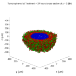
plot_cellular_automata( MCDS , 'Tumor spheroid at 3 weeks');
Simulation plots
Here are some plots, showing (left from right) pO2 concentration, a cross-section of the tumor (red = live cells, green = apoptotic, and blue = necrotic), and the drug concentration (after start of therapy):
1 week:

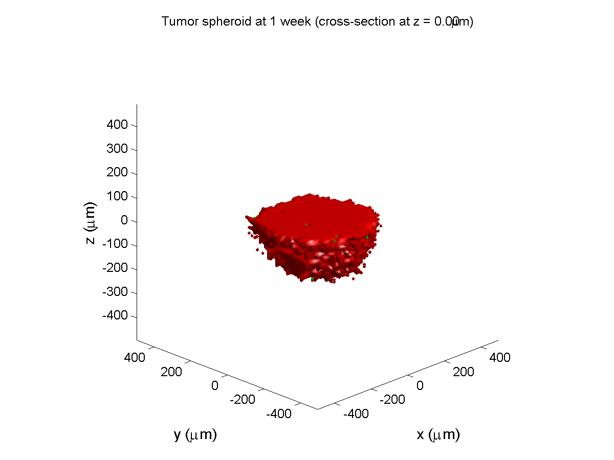
Oxygen- and space-limited growth are restricted to the outer boundary of the tumor spheroid.
2 weeks:
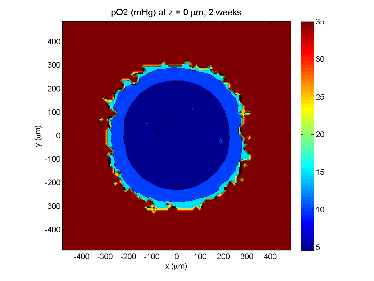
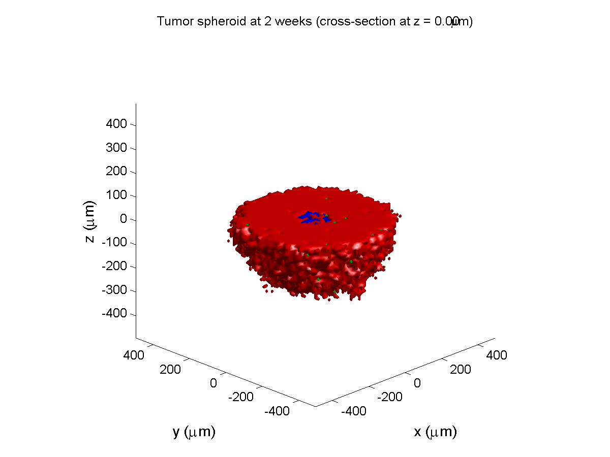
Oxygenation is dipped below 5 mmHg in the center, leading to necrosis.
3 weeks:
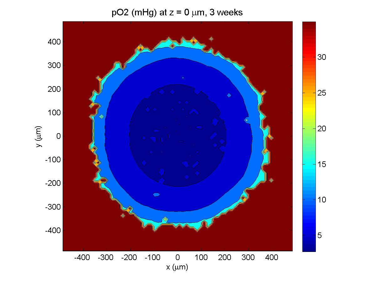
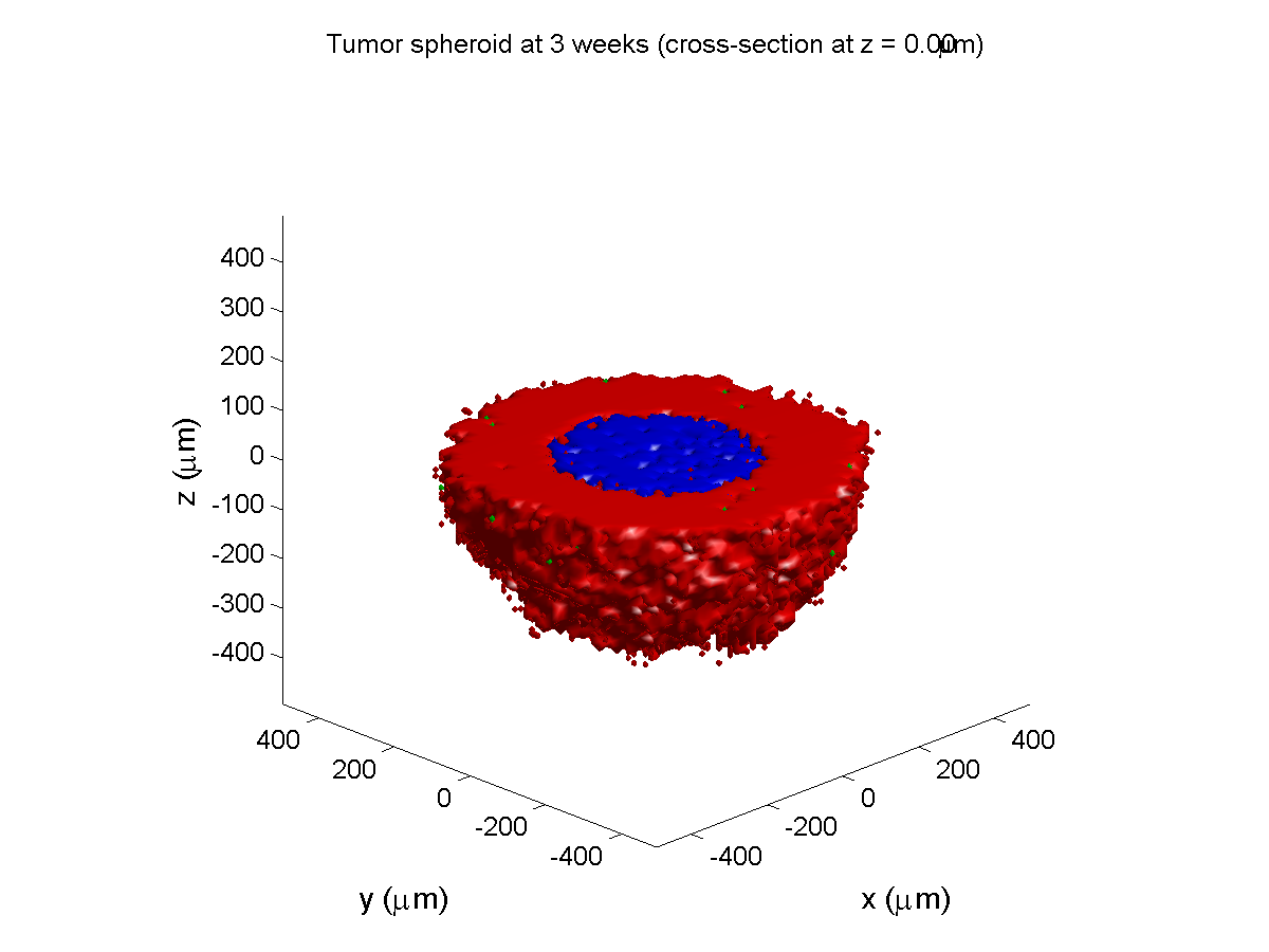
As the tumor grows, the hypoxic gradient increases, and the necrotic core grows. The code turns on a constant 5 micromolar dose of doxorubicin at this point
Treatment + 12 hours:
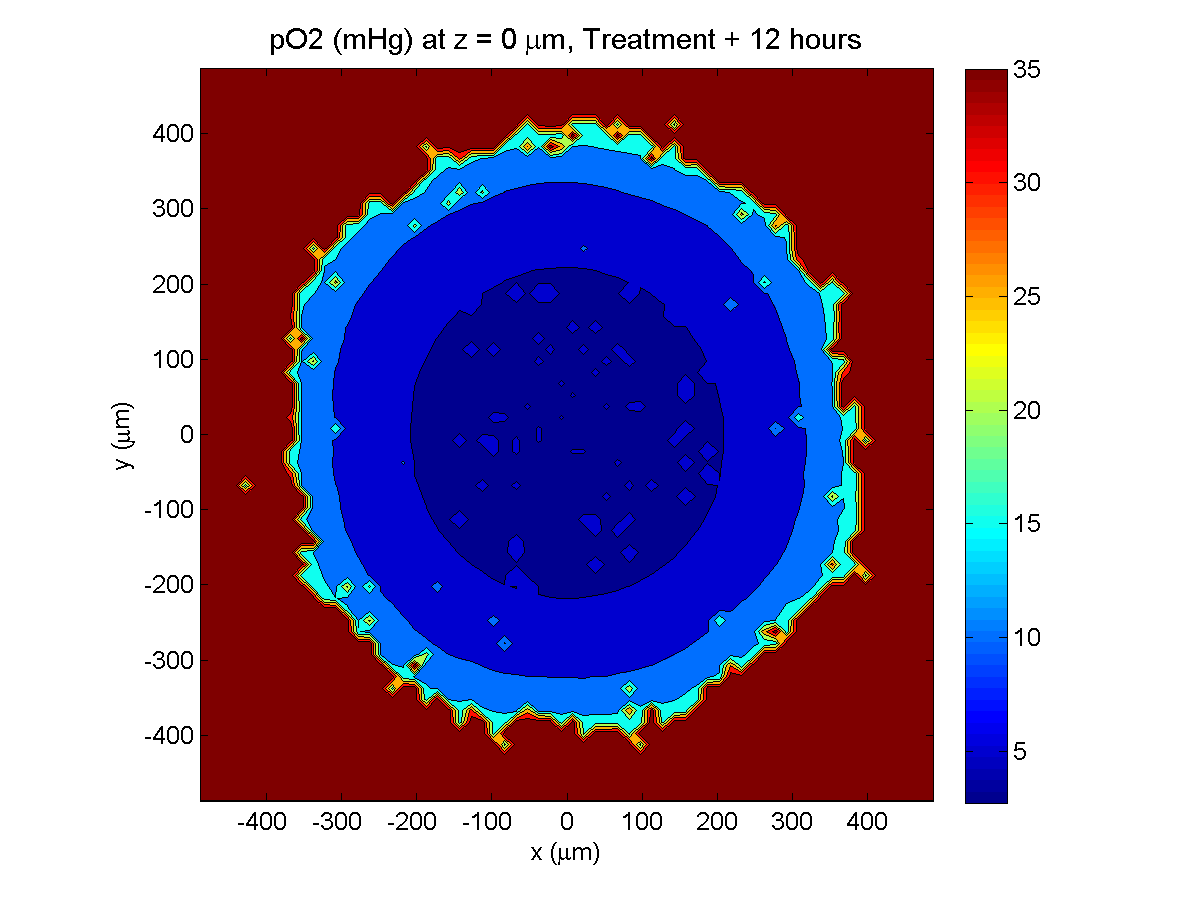
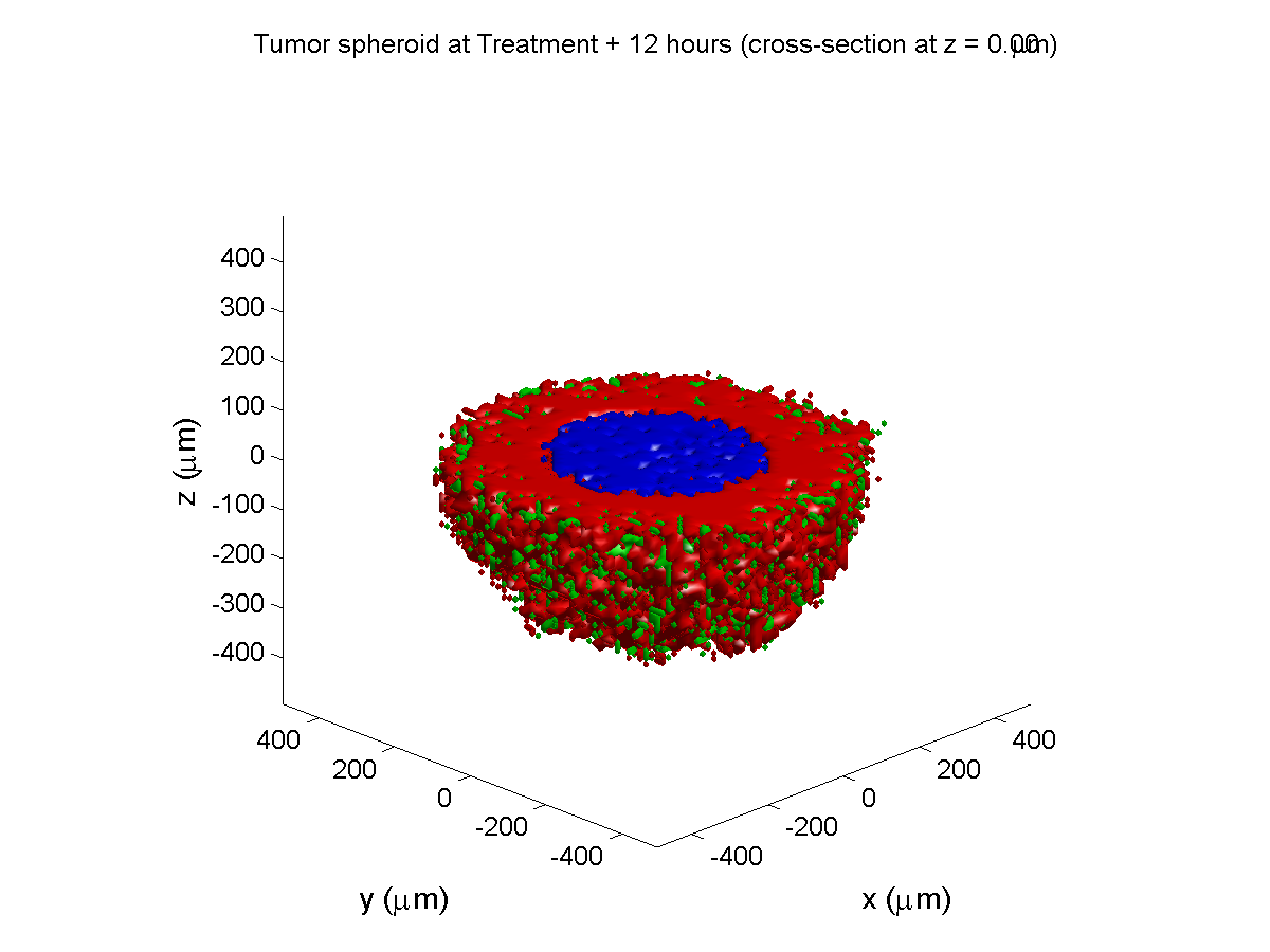

The drug has started to penetrate the tumor, triggering apoptotic death towards the outer periphery where exposure has been greatest.
Treatment + 24 hours:


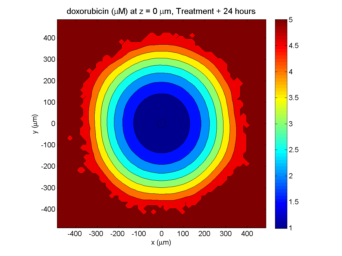
The drug profile hasn’t changed much, but the interior cells have now had greater exposure to drug, and hence greater response. Now apoptosis is observed throughout the non-necrotic tumor. The tumor has decreased in volume somewhat.
Treatment + 36 hours:
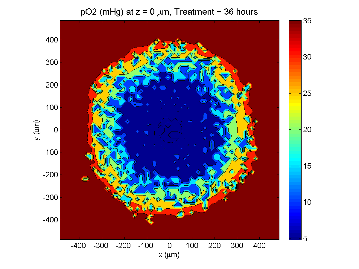
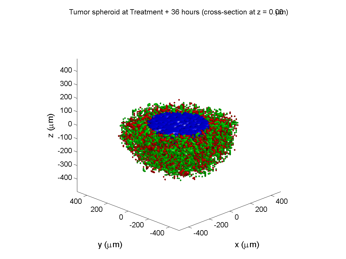
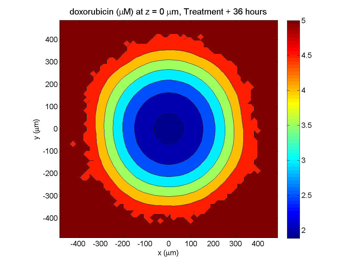
The non-necrotic tumor is now substantially apoptotic. We would require some pharamcokinetic effects (e.g., drug clearance, inactivation, or removal) to avoid the inevitable, presences of a pre-existing resistant strain, or emergence of resistance.
Treatment + 48 hours:
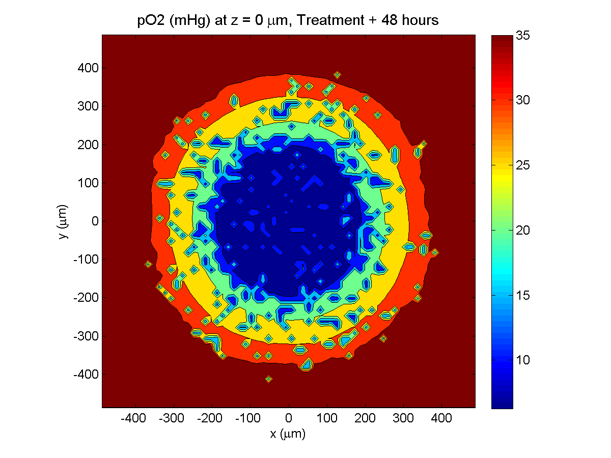
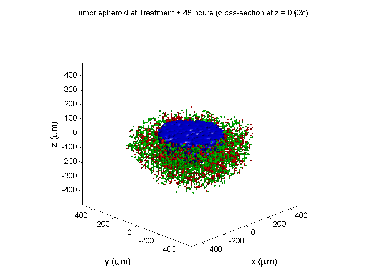
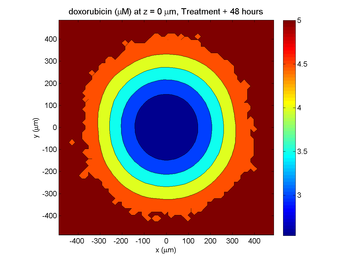
By now, almost all cells are apoptotic.
Treatment + 60 hours:

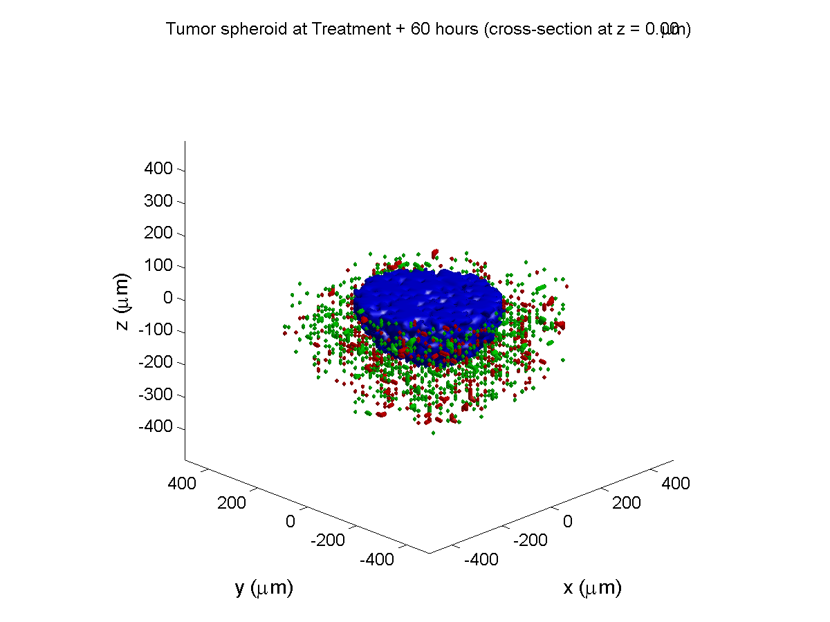

The non-necrotic tumor is nearly completed eliminated, leaving a leftover core of previously-necrotic cells (which did not change state in response to the drug–they were already dead!)
Source files
You can download completed source for this example here: https://sourceforge.net/projects/biofvm/files/Tutorials/Cellular_Automaton_1/
This file will include the following:
- BioFVM_cellular_automata.h
- BioFVM_cellular_automata.cpp
- BioFVM_CA_example_1.cpp
- read_MultiCellDS_xml.m (updated)
- plot_cellular_automata.m
- Makefile
What’s next
I plan to update this source code with extra cell motility, and potentially more realistic parameter values. Also, I plan to more formally separate out the example from the generic cell capabilities, so that this source code can work as a bona fide cellular automaton framework.
More immediately, my next tutorial will use the reverse strategy: start with an existing cellular automaton model, and integrate BioFVM capabilities.
Return to News • Return to MathCancer • Follow @MathCancer
Paul Macklin featured in Biotechniques article
Paul Macklin’s work on mathematical modeling of breast cancer and BioFVM was recently featured in Kelly Rae Chi’s article in Biotechniques on virtual cell cultures. It also included great work by James Glazier (CompuCell3D) and Kristin Swanson (glioblastoma modeling).
Read the article: http://www.biotechniques.com/news/Mighty-Modelers-The-Art-of-Virtual-Cell-Culture/biotechniques-364893.html (July 20, 2016)
Return to News • Return to MathCancer • Follow @MathCancer
Saving MultiCellDS data from BioFVM
Note: This is part of a series of “how-to” blog posts to help new users and developers of BioFVM.
Introduction
A major initiative for my lab has been MultiCellDS: a standard for multicellular data. The project aims to create model-neutral representations of simulation data (for both discrete and continuum models), which can also work for segmented experimental and clinical data. A single-time output is called a digital snapshot. An interdisciplinary, multi-institutional review panel has been hard at work to nail down the draft standard.
A BioFVM MultiCellDS digital snapshot includes program and user metadata (more information to be included in a forthcoming publication), an output of the microenvironment, and any cells that are secreting or uptaking substrates.
As of Version 1.1.0, BioFVM supports output saved to MultiCellDS XML files. Each download also includes a matlab function for importing MultiCellDS snapshots saved by BioFVM programs. This tutorial will get you going.
BioFVM (finite volume method for biological problems) is an open source code for solving 3-D diffusion of 1 or more substrates. It was recently published as open access in Bioinformatics here:
http://dx.doi.org/10.1093/bioinformatics/btv730
The project website is at http://BioFVM.MathCancer.org, and downloads are at http://BioFVM.sf.net.
Working with MultiCellDS in BioFVM programs
We include a MultiCellDS_test.cpp file in the examples directory of every BioFVM download (Version 1.1.0 or later). Create a new project directory, copy the following files to it:
- BioFVM*.cpp and BioFVM*.h (from the main BioFVM directory)
- pugixml.* (from the main BioFVM directory)
- Makefile and MultiCellDS_test.cpp (from the examples directory)
Open the MultiCellDS_test.cpp file to see the syntax as you read the rest of this post.
See earlier tutorials (below) if you have troubles with this.
Setting metadata values
There are few key bits of metadata. First, the program used for the simulation (all these fields are optional):
// the program name, version, and project website:
BioFVM_metadata.program.program_name = "BioFVM MultiCellDS Test";
BioFVM_metadata.program.program_version = "1.0";
BioFVM_metadata.program.program_URL = "http://BioFVM.MathCancer.org";

// who created the program (if known)
BioFVM_metadata.program.creator.surname = "Macklin";
BioFVM_metadata.program.creator.given_names = "Paul";
BioFVM_metadata.program.creator.email = "Paul.Macklin@usc.edu";
BioFVM_metadata.program.creator.URL = "http://BioFVM.MathCancer.org";
BioFVM_metadata.program.creator.organization = "University of Southern California";
BioFVM_metadata.program.creator.department = "Center for Applied Molecular Medicine";
BioFVM_metadata.program.creator.ORCID = "0000-0002-9925-0151";

// (generally peer-reviewed) citation information for the program
BioFVM_metadata.program.citation.DOI = "10.1093/bioinformatics/btv730";
BioFVM_metadata.program.citation.PMID = "26656933";
BioFVM_metadata.program.citation.PMCID = "PMC1234567";
BioFVM_metadata.program.citation.text = "A. Ghaffarizadeh, S.H. Friedman, and P. Macklin,
    BioFVM: an efficient parallelized diffusive transport solver for 3-D biological
    simulations, Bioinformatics, 2015. DOI: 10.1093/bioinformatics/btv730.";
BioFVM_metadata.program.citation.notes = "notes here";
BioFVM_metadata.program.citation.URL = "http://dx.doi.org/10.1093/bioinformatics/btv730";

// user information: who ran the program
BioFVM_metadata.program.user.surname = "Kirk";
BioFVM_metadata.program.user.given_names = "James T.";
BioFVM_metadata.program.user.email = "Jimmy.Kirk@starfleet.mil";
BioFVM_metadata.program.user.organization = "Starfleet";
BioFVM_metadata.program.user.department = "U.S.S. Enterprise (NCC 1701)";
BioFVM_metadata.program.user.ORCID = "0000-0000-0000-0000";

// And finally, data citation information (the publication where this simulation snapshot appeared)
BioFVM_metadata.data_citation.DOI = "10.1093/bioinformatics/btv730";
BioFVM_metadata.data_citation.PMID = "12345678";
BioFVM_metadata.data_citation.PMCID = "PMC1234567";
BioFVM_metadata.data_citation.text = "A. Ghaffarizadeh, S.H. Friedman, and P. Macklin, BioFVM:
    an efficient parallelized diffusive transport solver for 3-D biological simulations, Bioinformatics,
    2015. DOI: 10.1093/bioinformatics/btv730.";
BioFVM_metadata.data_citation.notes = "notes here";
BioFVM_metadata.data_citation.URL = "http://dx.doi.org/10.1093/bioinformatics/btv730";
You can sync the metadata current time, program runtime (wall time), and dimensional units using the following command. (This command is automatically run whenever you use the save command below.)
BioFVM_metadata.sync_to_microenvironment( M );
You can display a basic summary of the metadata via:
BioFVM_metadata.display_information( std::cout );
Setting options
By default (to save time and disk space), BioFVM saves the mesh as a Level 3 matlab file, whose location is embedded into the MultiCellDS XML file. You can disable this feature and revert to full XML (e.g., for human-readable cross-model reporting) via:
set_save_biofvm_mesh_as_matlab( false );
Similarly, BioFVM defaults to saving the values of the substrates in a compact Level 3 matlab file. You can override this with:
set_save_biofvm_data_as_matlab( false );
BioFVM by default saves the cell-centered sources and sinks. These take a lot of time to parse because they require very hierarchical data structures. You can disable saving the cells (basic_agents) via:
set_save_biofvm_cell_data( false );
Lastly, when you do save the cells, we default to a customized, minimal matlab format. You can revert to a more standard (but much larger) XML format with:
set_save_biofvm_cell_data_as_custom_matlab( false )
Saving a file
Saving the data is very straightforward:
save_BioFVM_to_MultiCellDS_xml_pugi( "sample" , M , current_simulation_time );
Your data will be saved in sample.xml. (Depending upon your options, it may generate several .mat files beginning with “sample”.)
If you’d like the filename to depend upon the simulation time, use something more like this:
double current_simulation_time = 10.347;
char filename_base [1024];
sprintf( &filename_base , "sample_%f", current_simulation_time );
save_BioFVM_to_MultiCellDS_xml_pugi( filename_base , M,
   current_simulation_time );
Your data will be saved in sample_10.347000.xml. (Depending upon your options, it may generate several .mat files beginning with “sample_10.347000”.)
Compiling and running the program:
Edit the Makefile as below:
PROGRAM_NAME := MCDS_test

all: $(BioFVM_OBJECTS) $(pugixml_OBJECTS) MultiCellDS_test.cpp

$(COMPILE_COMMAND) -o $(PROGRAM_NAME) $(BioFVM_OBJECTS) $(pugixml_OBJECTS) MultiCellDS_test.cpp
If you’re running OSX, you’ll probably need to update the compiler from “g++”. See these tutorials.
Then, at the command prompt:
make
./MCDS_test
On Windows, you’ll need to run without the ./:
make
MCDS_test
Working with MultiCellDS data in Matlab
Reading data in Matlab
Copy the read_MultiCellDS_xml.m file from the matlab directory (included in every MultiCellDS download). To read the data, just do this:
MCDS = read_MultiCellDS_xml( 'sample.xml' );
This should take around 30 seconds for larger data files (500,000 to 1,000,000 voxels with a few substrates, and around 250,000 cells). The long execution time is primarily because Matlab is ghastly inefficient at loops over hierarchical data structures. Increasing to 1,000,000 cells requires around 80-90 seconds to parse in matlab.
Plotting data in Matlab
Plotting the 3-D substrate data
First, let’s do some basic contour and surface plotting:
mid_index = round( length(MCDS.mesh.Z_coordinates)/2 );

contourf( MCDS.mesh.X(:,:,mid_index), ...
	MCDS.mesh.Y(:,:,mid_index), ...
	MCDS.continuum_variables(2).data(:,:,mid_index) , 20 ) ;
axis image
colorbar
xlabel( sprintf( 'x (%s)' , MCDS.metadata.spatial_units) );
ylabel( sprintf( 'y (%s)' , MCDS.metadata.spatial_units) );
title( sprintf('%s (%s) at t = %f %s, z = %f %s', MCDS.continuum_variables(2).name , ...
	MCDS.continuum_variables(2).units , ...
	MCDS.metadata.current_time , ...
	MCDS.metadata.time_units, ...
	MCDS.mesh.Z_coordinates(mid_index), ...
	MCDS.metadata.spatial_units ) );
OR
contourf( MCDS.mesh.X_coordinates , MCDS.mesh.Y_coordinates, ...
	MCDS.continuum_variables(2).data(:,:,mid_index) , 20 ) ;
axis image
colorbar
xlabel( sprintf( 'x (%s)' , MCDS.metadata.spatial_units) );
ylabel( sprintf( 'y (%s)' , MCDS.metadata.spatial_units) );
title( sprintf('%s (%s) at t = %f %s, z = %f %s', ...
	MCDS.continuum_variables(2).name , ...
	MCDS.continuum_variables(2).units , ...
	MCDS.metadata.current_time , ...
	MCDS.metadata.time_units, ...
	MCDS.mesh.Z_coordinates(mid_index), ...
	MCDS.metadata.spatial_units ) );
Here’s a surface plot:
surf( MCDS.mesh.X_coordinates , MCDS.mesh.Y_coordinates, ...
	MCDS.continuum_variables(1).data(:,:,mid_index) ) ;
colorbar
axis tight
xlabel( sprintf( 'x (%s)' , MCDS.metadata.spatial_units) );
ylabel( sprintf( 'y (%s)' , MCDS.metadata.spatial_units) );
zlabel( sprintf( '%s (%s)', MCDS.continuum_variables(1).name, ...
	MCDS.continuum_variables(1).units ) );
title( sprintf('%s (%s) at t = %f %s, z = %f %s', MCDS.continuum_variables(1).name , ...
	MCDS.continuum_variables(1).units , ...
	MCDS.metadata.current_time , ...
	MCDS.metadata.time_units, ...
	MCDS.mesh.Z_coordinates(mid_index), ...
	MCDS.metadata.spatial_units ) );
Finally, here are some more advanced plots. The first is an “exploded” stack of contour plots:
clf
contourslice( MCDS.mesh.X , MCDS.mesh.Y, MCDS.mesh.Z , ...
	MCDS.continuum_variables(2).data , [],[], ...
	MCDS.mesh.Z_coordinates(1:15:length(MCDS.mesh.Z_coordinates)),20);
view([-45 10]);
axis tight;
xlabel( sprintf( 'x (%s)' , MCDS.metadata.spatial_units) );
ylabel( sprintf( 'y (%s)' , MCDS.metadata.spatial_units) );
zlabel( sprintf( 'z (%s)' , MCDS.metadata.spatial_units) );
title( sprintf('%s (%s) at t = %f %s', ...
	MCDS.continuum_variables(2).name , ...
	MCDS.continuum_variables(2).units , ...
	MCDS.metadata.current_time, ...
	MCDS.metadata.time_units ) );
Next, we show how to use isosurfaces with transparency
clf
patch( isosurface( MCDS.mesh.X , MCDS.mesh.Y, MCDS.mesh.Z, ...
	MCDS.continuum_variables(1).data, 1000 ), 'edgecolor', ...
	'none', 'facecolor', 'r' , 'facealpha' , 1 );
hold on
patch( isosurface( MCDS.mesh.X , MCDS.mesh.Y, MCDS.mesh.Z, ...
MCDS.continuum_variables(1).data, 5000 ), 'edgecolor', ...
	'none', 'facecolor', 'b' , 'facealpha' , 0.7 );
patch( isosurface( MCDS.mesh.X , MCDS.mesh.Y, MCDS.mesh.Z, ...
	MCDS.continuum_variables(1).data, 10000 ), 'edgecolor', ...
	'none', 'facecolor', 'g' , 'facealpha' , 0.5 );
hold off
% shading interp
camlight
view(3)
axis image
axis tightcamlight lighting gouraud
xlabel( sprintf( 'x (%s)' , MCDS.metadata.spatial_units) );
ylabel( sprintf( 'y (%s)' , MCDS.metadata.spatial_units) );
zlabel( sprintf( 'z (%s)' , MCDS.metadata.spatial_units) );
title( sprintf('%s (%s) at t = %f %s', ...
	MCDS.continuum_variables(1).name , ...
	MCDS.continuum_variables(1).units , ...
	MCDS.metadata.current_time, ...
	MCDS.metadata.time_units ) );
You can get more 3-D volumetric visualization ideas at Matlab’s website. This visualization post at MIT also has some great tips.
Plotting the cells
Here is a basic 3-D plot for the cells:
plot3( MCDS.discrete_cells.state.position(:,1) , ...
	MCDS.discrete_cells.state.position(:,2) , ...
	MCDS.discrete_cells.state.position(:,3) , 'bo' );
view(3)
axis tight
xlabel( sprintf( 'x (%s)' , MCDS.metadata.spatial_units) );
ylabel( sprintf( 'y (%s)' , MCDS.metadata.spatial_units) );
zlabel( sprintf( 'z (%s)' , MCDS.metadata.spatial_units) );
title( sprintf('Cells at t = %f %s', MCDS.metadata.current_time, ...
	MCDS.metadata.time_units ) );
plot3 is more efficient than scatter3, but scatter3 will give more coloring options. Here is the syntax:
scatter3( MCDS.discrete_cells.state.position(:,1), ...
	MCDS.discrete_cells.state.position(:,2), ...
	MCDS.discrete_cells.state.position(:,3) , 'bo' );
view(3)
axis tight
xlabel( sprintf( 'x (%s)' , MCDS.metadata.spatial_units) );
ylabel( sprintf( 'y (%s)' , MCDS.metadata.spatial_units) );
zlabel( sprintf( 'z (%s)' , MCDS.metadata.spatial_units) );
title( sprintf('Cells at t = %f %s', MCDS.metadata.current_time, ...
	MCDS.metadata.time_units ) );
Jan Poleszczuk gives some great insights on plotting many cells in 3D at his blog. I’d recommend checking out his post on visualizing a cellular automaton model. At some point, I’ll update this post with prettier plotting based on his methods.
What’s next
Future releases of BioFVM will support reading MultiCellDS snapshots (for model initialization).
Matlab is pretty slow at parsing and visualizing large amounts of data. We also plan to include resources for accessing MultiCellDS data in VTK / Paraview and Python.
Return to News • Return to MathCancer • Follow @MathCancer
BioFVM warmup: 2D continuum simulation of tumor growth
Note: This is part of a series of “how-to” blog posts to help new users and developers of BioFVM. See also the guides to setting up a C++ compiler in Windows or OSX.
What you’ll need
- A working C++ development environment with support for OpenMP. See these prior tutorials if you need help.
- A download of BioFVM, available at http://BioFVM.MathCancer.org and http://BioFVM.sf.net. Use Version 1.0.3 or later.
- Matlab or Octave for visualization. Matlab might be available for free at your university. Octave is open source and available from a variety of sources.
Our modeling task
We will implement a basic 2-D model of tumor growth in a heterogeneous microenvironment, with inspiration by glioblastoma models by Kristin Swanson, Russell Rockne and others (e.g., this work), and continuum tumor growth models by Hermann Frieboes, John Lowengrub, and our own lab (e.g., this paper and this paper).
We will model tumor growth driven by a growth substrate, where cells die when the growth substrate is insufficient. The tumor cells will have motility. A continuum blood vasculature will supply the growth substrate, but tumor cells can degrade this existing vasculature. We will revisit and extend this model from time to time in future tutorials.
Mathematical model
Taking inspiration from the groups mentioned above, we’ll model a live cell density ρ of a relatively low-adhesion tumor cell species (e.g., glioblastoma multiforme). We’ll assume that tumor cells move randomly towards regions of low cell density (modeled as diffusion with motility μ). We’ll assume that that the net birth rate rB is proportional to the concentration of growth substrate σ, which is released by blood vasculature with density b. Tumor cells can degrade the tissue and hence this existing vasculature. Tumor cells die at rate rD when the growth substrate level is too low. We assume that the tumor cell density cannot exceed a max level ρmax. A model that includes these effects is:
\[ \frac{ \partial \rho}{\partial t} = \mu \nabla^2 \rho + r_B(\sigma)\rho \left( 1 – \frac{ \rho}{\rho_\textrm{max}} \right) – r_D(\sigma) \rho \]
\[ \frac{ \partial b}{\partial t} = – r_\textrm{degrade} \rho b \]
\[ \frac{\partial \sigma}{ \partial t} = D\nabla^2 \sigma – \lambda_a \sigma – \lambda_2 \rho \sigma + r_\textrm{deliv}b \left( \sigma_\textrm{max} – \sigma \right) \]
where for the birth and death rates, we’ll use the constitutive relations:
\[ r_B(\sigma) = r_B \textrm{ max} \left( \frac{\sigma – \sigma_\textrm{min}}{ \sigma_\textrm{ max} – \sigma_\textrm{min} } , 0 \right)\]
\[r_D(\sigma) = r_D \textrm{ max} \left( \frac{ \sigma_\textrm{min} – \sigma}{\sigma_\textrm{min}} , 0 \right) \]
Mapping the model onto BioFVM
BioFVM solves on a vector u of substrates. We’ll set u = [ρ , b, σ ]. The code expects PDEs of the general form:
\[ \frac{\partial q}{\partial t} = D\nabla^2 q – \lambda q + S\left( q^* – q \right) – Uq\]
So, we determine the decay rate (λ), source function (S), and uptake function (U) for the cell density ρ and the growth substrate σ.
Cell density
We first slightly rewrite the PDE:
\[ \frac{ \partial \rho}{\partial t} = \mu \nabla^2 \rho + r_B(\sigma) \frac{ \rho}{\rho_\textrm{max}} \left( \rho_\textrm{max} – \rho \right) – r_D(\sigma)\rho \]
and then try to match to the general form term-by-term. While BioFVM wasn’t intended for solving nonlinear PDEs of this form, we can make it work by quasi-linearizing, with the following functions:
\[ S = r_B(\sigma) \frac{ \rho }{\rho_\textrm{max}} \hspace{1in} U = r_D(\sigma). \]
When implementing this, we’ll evaluate σ and ρ at the previous time step. The diffusion coefficient is μ, and the decay rate is zero. The target or saturation density is ρmax.
Growth substrate
Similarly, by matching the PDE for σ term-by-term with the general form, we use:
\[ S = r_\textrm{deliv}b, \hspace{1in} U = \lambda_2 \rho. \]
The diffusion coefficient is D, the decay rate is λ1, and the saturation density is σmax.
Blood vessels
Lastly, a term-by-term matching of the blood vessel equation gives the following functions:
\[ S=0 \hspace{1in} U = r_\textrm{degrade}\rho. \]
The diffusion coefficient, decay rate, and saturation density are all zero.
Implementation in BioFVM
- Start a project: Create a new directory for your project (I’d recommend “BioFVM_2D_tumor”), and enter the directory. Place a copy of BioFVM (the zip file) into your directory. Unzip BioFVM, and copy BioFVM*.h, BioFVM*.cpp, and pugixml* files into that directory.
- Copy the matlab visualization files: To help read and plot BioFVM data, we have provided matlab files. Copy all the *.m files from the matlab subdirectory to your project.
- Copy the empty project: BioFVM Version 1.0.3 or later includes a template project and Makefile to make it easier to get started. Copy the Makefile and template_project.cpp file to your project. Rename template_project.cpp to something useful, like 2D_tumor_example.cpp.
- Edit the makefile: Open a terminal window and browse to your project. Tailor the makefile to your new project:
notepad++ Makefile
Change the PROGRAM_NAME to 2Dtumor.
Also, rename main to 2D_tumor_example throughout the Makefile.
Lastly, note that if you are using OSX, you’ll probably need to change from “g++” to your installed compiler. See these tutorials.
- Start adapting 2D_tumor_example.cpp: First, open 2D_tumor_example.cpp:
notepad++ 2D_tumor_example.cpp
Just after the “using namespace BioFVM” section of the code, define useful globals. Here and throughout, new and/or modified code is in blue:
using namespace BioFVM:

// helpful -- have indices for each "species"
int live_cells  = 0;
int blood_vessels = 1;
int oxygen    = 2;

// some globals
double prolif_rate = 1.0 /24.0;
double death_rate = 1.0 / 6; //
double cell_motility = 50.0 / 365.25 / 24.0 ;
// 50 mm^2 / year --> mm^2 / hour
double o2_uptake_rate = 3.673 * 60.0; // 165 micron length scale
double vessel_degradation_rate = 1.0 / 2.0 / 24.0 ;
// 2 days to disrupt tissue

double max_cell_density = 1.0;

double o2_supply_rate = 10.0;
double o2_normoxic  = 1.0;
double o2_hypoxic   = 0.2;
- Set up the microenvironment: Within main(), make sure we have the right number of substrates, and set them up:
// create a microenvironment, and set units

Microenvironment M;
M.name = "Tumor microenvironment";
M.time_units = "hr";
M.spatial_units = "mm";
M.mesh.units = M.spatial_units;

// set up and add all the densities you plan

M.set_density( 0 , "live cells" , "cells" );
M.add_density( "blood vessels" , "vessels/mm^2" );
M.add_density( "oxygen" , "cells" );

// set the properties of the diffusing substrates

M.diffusion_coefficients[live_cells] = cell_motility;

M.diffusion_coefficients[blood_vessels] = 0;
M.diffusion_coefficients[oxygen] = 6.0;

// 1e5 microns^2/min in units mm^2 / hr

M.decay_rates[live_cells] = 0;
M.decay_rates[blood_vessels] = 0;
M.decay_rates[oxygen] = 0.01 * o2_uptake_rate;
// 1650 micron length scale
Notice how our earlier global definitions of “live_cells”, “blood_vessels”, and “oxygen” makes it easier to make sure we’re referencing the correct substrates in lines like these.
- Resize the domain and test: For this example (and so the code runs very quickly), we’ll work in 2D in a 2 cm × 2 cm domain:
// set the mesh size

double dx = 0.05; // 50 microns
M.resize_space( 0.0 , 20.0 , 0, 20.0 , -dx/2.0, dx/2.0 , dx, dx, dx );
Notice that we use a tissue thickness of dx/2 to use the 3D code for a 2D simulation. Now, let’s test:
make
2Dtumor
Go ahead and cancel the simulation [Control]+C after a few seconds. You should see something like this:
Starting program ...

Microenvironment summary: Tumor microenvironment:

Mesh information:
type: uniform Cartesian
Domain: [0,20] mm x [0,20] mm x [-0.025,0.025] mm
	resolution: dx = 0.05 mm
	voxels: 160000
	voxel faces: 0
	volume: 20 cubic mm
Densities: (3 total)
	live cells:
	units: cells
	diffusion coefficient: 0.00570386 mm^2 / hr
	decay rate: 0 hr^-1
	diffusion length scale: 75523.9 mm

	blood vessels:
	units: vessels/mm^2
	diffusion coefficient: 0 mm^2 / hr
	decay rate: 0 hr^-1
	diffusion length scale: 0 mm

	oxygen:
	units: cells
	diffusion coefficient: 6 mm^2 / hr
	decay rate: 2.2038 hr^-1
	diffusion length scale: 1.65002 mm

simulation time: 0 hr (100 hr max)

Using method diffusion_decay_solver__constant_coefficients_LOD_3D (implicit 3-D LOD with Thomas Algorithm) ...

simulation time: 10 hr (100 hr max)
simulation time: 20 hr (100 hr max)
- Set up initial conditions: We’re going to make a small central focus of tumor cells, and a “bumpy” field of blood vessels.
// set initial conditions // use this syntax to create a zero vector of length 3 // std::vector<double> zero(3,0.0); std::vector<double> center(3); center[0] = M.mesh.x_coordinates[M.mesh.x_coordinates.size()-1] /2.0; center[1] = M.mesh.y_coordinates[M.mesh.y_coordinates.size()-1] /2.0; center[2] = 0; double radius = 1.0; std::vector<double> one( M.density_vector(0).size() , 1.0 ); double pi = 2.0 * asin( 1.0 ); // use this syntax for a parallelized loop over all the // voxels in your mesh: #pragma omp parallel for for( int i=0; i < M.number_of_voxels() ; i++ ) { std::vector<double> displacement = M.voxels(i).center – center; double distance = norm( displacement ); if( distance < radius ) { M.density_vector(i)[live_cells] = 0.1; } M.density_vector(i)[blood_vessels]= 0.5 + 0.5*cos(0.4* pi * M.voxels(i).center[0])*cos(0.3*pi *M.voxels(i).center[1]); M.density_vector(i)[oxygen] = o2_normoxic; } - Change to a 2D diffusion solver:
// set up the diffusion solver, sources and sinks

M.diffusion_decay_solver = diffusion_decay_solver__constant_coefficients_LOD_2D;
- Set the simulation times: We’ll simulate 10 days, with output every 12 hours.
double t = 0.0;
double t_max = 10.0 * 24.0; // 10 days
double dt = 0.1;

double output_interval = 12.0; // how often you save data
double next_output_time = t; // next time you save data
- Set up the source function:
void supply_function( Microenvironment* microenvironment, int voxel_index, std::vector<double>* write_here )
{
	// use this syntax to access the jth substrate write_here
	// (*write_here)[j]
	// use this syntax to access the jth substrate in voxel voxel_index of microenvironment:
	// microenvironment->density_vector(voxel_index)[j]

	static double temp1 = prolif_rate / ( o2_normoxic – o2_hypoxic );

	(*write_here)[live_cells] =
		microenvironment->density_vector(voxel_index)[oxygen];
	(*write_here)[live_cells] -= o2_hypoxic;

	if( (*write_here)[live_cells] < 0.0 )
	{
		(*write_here)[live_cells] = 0.0;
	}
	else
	{
		(*write_here)[live_cells] = temp1;
		(*write_here)[live_cells] *=
			microenvironment->density_vector(voxel_index)[live_cells];
	}

	(*write_here)[blood_vessels] = 0.0;
	(*write_here)[oxygen] = o2_supply_rate;
	(*write_here)[oxygen] *=
		microenvironment->density_vector(voxel_index)[blood_vessels];

	return;
}
Notice the use of the static internal variable temp1: the first time this function is called, it declares this helper variable (to save some multiplication operations down the road). The static variable is available to all subsequent calls of this function.
- Set up the target function (substrate saturation densities):
void supply_target_function( Microenvironment* microenvironment, int voxel_index, std::vector<double>* write_here ) { // use this syntax to access the jth substrate write_here // (*write_here)[j] // use this syntax to access the jth substrate in voxel voxel_index of microenvironment: // microenvironment->density_vector(voxel_index)[j] (*write_here)[live_cells] = max_cell_density; (*write_here)[blood_vessels] = 1.0; (*write_here)[oxygen] = o2_normoxic; return; } - Set up the uptake function:
void uptake_function( Microenvironment* microenvironment, int voxel_index,
	std::vector<double>* write_here )
{
	// use this syntax to access the jth substrate write_here
	// (*write_here)[j]
	// use this syntax to access the jth substrate in voxel voxel_index of microenvironment:
	// microenvironment->density_vector(voxel_index)[j]

	(*write_here)[live_cells] = o2_hypoxic;
	(*write_here)[live_cells] -=
		microenvironment->density_vector(voxel_index)[oxygen];
	if( (*write_here)[live_cells] < 0.0 )
	{
		(*write_here)[live_cells] = 0.0;
	}
	else
	{
		(*write_here)[live_cells] *= death_rate;
	}

	(*write_here)[oxygen] = o2_uptake_rate ;
	(*write_here)[oxygen] *=
		microenvironment->density_vector(voxel_index)[live_cells];

	(*write_here)[blood_vessels] = vessel_degradation_rate ;
	(*write_here)[blood_vessels] *=
		microenvironment->density_vector(voxel_index)[live_cells];

	return;
}
And that’s it. The source should be ready to go!
Source files
You can download completed source for this example here:
Using the code
Running the code
First, compile and run the code:
make
2Dtumor
The output should look like this.
Starting program …

Microenvironment summary: Tumor microenvironment:

Mesh information:
type: uniform Cartesian
Domain: [0,20] mm x [0,20] mm x [-0.025,0.025] mm
	resolution: dx = 0.05 mm
	voxels: 160000
	voxel faces: 0
	volume: 20 cubic mm
Densities: (3 total)
	live cells:
		units: cells
		diffusion coefficient: 0.00570386 mm^2 / hr
		decay rate: 0 hr^-1
		diffusion length scale: 75523.9 mm

	blood vessels:
		units: vessels/mm^2
		diffusion coefficient: 0 mm^2 / hr
		decay rate: 0 hr^-1
		diffusion length scale: 0 mm

	oxygen:
		units: cells
		diffusion coefficient: 6 mm^2 / hr
		decay rate: 2.2038 hr^-1
		diffusion length scale: 1.65002 mm

simulation time: 0 hr (240 hr max)

Using method diffusion_decay_solver__constant_coefficients_LOD_2D (2D LOD with Thomas Algorithm) …

simulation time: 12 hr (240 hr max)
simulation time: 24 hr (240 hr max)
simulation time: 36 hr (240 hr max)
simulation time: 48 hr (240 hr max)
simulation time: 60 hr (240 hr max)
simulation time: 72 hr (240 hr max)
simulation time: 84 hr (240 hr max)
simulation time: 96 hr (240 hr max)
simulation time: 108 hr (240 hr max)
simulation time: 120 hr (240 hr max)
simulation time: 132 hr (240 hr max)
simulation time: 144 hr (240 hr max)
simulation time: 156 hr (240 hr max)
simulation time: 168 hr (240 hr max)
simulation time: 180 hr (240 hr max)
simulation time: 192 hr (240 hr max)
simulation time: 204 hr (240 hr max)
simulation time: 216 hr (240 hr max)
simulation time: 228 hr (240 hr max)
simulation time: 240 hr (240 hr max)
Done!
Looking at the data
Now, let’s pop it open in matlab (or octave):
matlab
To load and plot a single time (e.g., the last tim)
!ls *.mat
M = read_microenvironment( 'output_240.000000.mat' );
plot_microenvironment( M );
To add some labels:
labels{1} = 'tumor cells';
labels{2} = 'blood vessel density';
labels{3} = 'growth substrate';
plot_microenvironment( M ,labels );
Your output should look a bit like this:

Lastly, you might want to script the code to create and save plots of all the times.
labels{1} = 'tumor cells';
labels{2} = 'blood vessel density';
labels{3} = 'growth substrate';
for i=0:20
	t = i*12;
	input_file = sprintf( 'output_%3.6f.mat', t );
	output_file = sprintf( 'output_%3.6f.png', t );
	M = read_microenvironment( input_file );
	plot_microenvironment( M , labels );
	print( gcf , '-dpng' , output_file );
end
What’s next
We’ll continue posting new tutorials on adapting BioFVM to existing and new simulators, as well as guides to new features as we roll them out.
Stay tuned and watch this blog!
Setting up gcc / OpenMP on OSX (Homebrew edition)
Note: This is part of a series of “how-to” blog posts to help new users and developers of BioFVM and PhysiCell. This guide is for OSX users. Windows users should use this guide instead. A Linux guide is expected soon.
These instructions should get you up and running with a minimal environment for compiling 64-bit C++ projects with OpenMP (e.g., BioFVM and PhysiCell) using gcc. These instructions were tested with OSX 10.11 (El Capitan) and 10.12 (Sierra), but they should work on any reasonably recent version of OSX.
In the end result, you’ll have a compiler and key makefile capabilities. The entire toolchain is free and open source.
Of course, you can use other compilers and more sophisticated integrated desktop environments, but these instructions will get you a good baseline system with support for 64-bit binaries and OpenMP parallelization.
Note 1: OSX / Xcode appears to have gcc out of the box (you can type “gcc” in a Terminal window), but this really just maps back onto Apple’s build of clang. Alas, this will not support OpenMP for parallelization.
Note 2: In this post, we showed how to set up gcc using the popular MacPorts package manager. Because MacPorts builds gcc (and all its dependencies!) from source, it takes a very, very long time. On my 2012 Macbook Air, this step took 16 hours. This tutorial uses Homebrew to dramatically speed up the process!
Note 3: This is an update over the previous version. It incorporates new information that Xcode command line tools can be installed without the full 4.41 GB download / installation of Xcode. Many thanks to Walter de Back and Tim at the Homebrew project for their help!
What you’ll need:
- XCode Command Line Tools: These command line tools are needed for Homebrew and related package managers. Installation instructions are now very simple and included below. As of January 18, 2016, this will install Version 2343.
- Homebrew: This is a package manager for OSX, which will let you easily download and install many linux utilities without building them from source. You’ll particularly need it for getting gcc. Installation is a simple command-line script, as detailed below. As of August 2, 2017, this will download Version 1.3.0.
- gcc (from Homebrew): This will be an up-to-date 64-bit version of gcc, with support for OpenMP. As of August 2, 2017, this will download Version 7.1.0.
Main steps:
1) Install the XCode Command Line Tools
Open a terminal window (Open Launchpad, then “Other”, then “Terminal”), and run:
user$ xcode-select --install
A window should pop up asking you to either get Xcode or install. Choose the “install” option to avoid the huge 4+ GB Xcode download. It should only take a few minutes to complete.
2) Install Homebrew
Open a terminal window (Open Launchpad, then “Other”, then “Terminal”), and run:
user$ ruby -e "$(curl -fsSL https://raw.githubusercontent.com/Homebrew/install/master/install)"
Let the script run, and answer “y” whenever asked. This will not take very long.
3) Get, install, and prepare gcc
Open a terminal window (see above), and search for gcc, version 7.x or above
user$ brew search gcc
You should see a list of packages, including gcc7. (In 2015, this looked like “gcc5”. In 2017, this looks like “gcc@7”.)
Then, download and install gcc:
user$ brew install gcc
This will download whatever dependencies are needed, generally already pre-compiled. The whole process should only take five or ten minutes.
Lastly, you need to get the exact name of your compiler. In your terminal window, type g++, and then hit tab twice to see a list. On my system, I see this:
Pauls-MBA:~ pmacklin$ g++
g++       g++-7     g++-mp-7
Look for the version of g++ without an “mp” (from MacPorts) in its name. In my case, it’s g++-7. Double-check that you have the right one by checking its version. It should look something like this:
Pauls-MBA:~ pmacklin$ g++-7 --version
g++-7 (Homebrew GCC 7.1.0) 7.1.0
Copyright (C) 2017 Free Software Foundation, Inc.
This is free software; see the source for copying conditions.  There is NO warranty; not even
for MERCHANTABILITY or FITNESS FOR A PARTICULAR PURPOSE.
Notice that Homebrew shows up in the information. The correct compiler is g++-7.
PhysiCell Version 1.2.2 and greater use a system variable to record your compiler version, so that you don’t need to modify the CC line in PhysiCell Makefiles. Set the PHYSICELL_CPP variable to record the compiler you just found above. For example, on the bash shell:
export PHYSICELL_CPP=g++-7
echo export PHYSICELL_CPP=g++-7 >> ~/.bash_profile
One last thing: If you don’t update your paths, make will may fail as it continues to combine Apple’s “gcc” toolchain with real gcc. (This seems to happen most often if you installed an older gcc like gcc5 with MacPorts earlier.) You may see errors like this:
user$ make
g++-7 -march=core2 -O3 -fomit-frame-pointer -fopenmp -std=c++11 -c BioFVM_vector.cpp
FATAL:/opt/local/bin/../libexec/as/x86_64/as: I don't understand 'm' flag!
make: *** [BIOFVM_vector.o] Error 1
To avoid this, run:
echo export PATH=/usr/local/bin:$PATH >> ~/.bash_profile
Note that you’ll need to open a new Terminal window for this fix to apply.
4) Test your setup
I wrote a sample C++ program that tests OpenMP parallelization (32 threads). If you can compile and run it, it means that everything (including make) is working! :-)
Make a new directory, and enter it
Open Terminal (see above). You should be in your user profile’s root directory. Make a new subdirectory called GCC_test, and enter it.
mkdir GCC_test
cd GCC_test
Grab a sample parallelized program:
Download a Makefile and C++ source file, and save them to the GCC_test directory. Here are the links:
- Makefile: [click here]
- C++ source: [click here]
Note: The Makefiles in PhysiCell (versions > 1.2.1) can use an environment variable to specify an OpenMP-capable g++ compiler. If you have not yet done so, you should go ahead and set that now, e.g., for the bash shell:
export PHYSICELL_CPP=g++-7
echo export PHYSICELL_CPP=g++-7 >> ~/.bash_profile
Compile and run the test:
Go back to your (still open) command prompt. Compile and run the program:
make
./my_test
The output should look something like this:
Allocating 4096 MB of memory ...
Done!

Entering main loop ...
Done!
Note 1: If the make command gives errors like “**** missing separator”, then you need to replace the white space (e.g., one or more spaces) at the start of the “$(COMPILE_COMMAND)” and “rm -f” lines with a single tab character.
Note 2: If the compiler gives an error like “fatal error: ‘omp.h’ not found”, you probably used Apple’s build of clang, which does not include OpenMP support. You’ll need to make sure that you set the environment variable PHYSICELL_CPP as above (for PhysiCell 1.2.2 or later), or specify your compiler on the CC line of your makefile (for PhysiCell 1.2.1 or earlier).
Now, let’s verify that the code is using OpenMP.
Open another Terminal window. While the code is running, run top. Take a look at the performance, particularly CPU usage. While your program is running, you should see CPU usage fairly close to ‘100% user’. (This is a good indication that your code is running the OpenMP parallelization as expected.)
What’s next?
Download a copy of PhysiCell and try out the included examples! Visit BioFVM at MathCancer.org.
- PhysiCell links:
- PhysiCell Method Paper at bioRxiv: https://doi.org/10.1101/088773
- PhysiCell on MathCancer: http://PhysiCell.MathCancer.org
- PhysiCell on SourceForge: http://PhysiCell.sf.net
- PhysiCell on github: http://github.com/MathCancer/PhysiCell
- PhysiCell tutorials: [click here]
- BioFVM links:
- BioFVM announcement on this blog: [click here]
- BioFVM on MathCancer.org: http://BioFVM.MathCancer.org
- BioFVM on SourceForge: http://BioFVM.sf.net
- BioFVM Method Paper in BioInformatics: http://dx.doi.org/10.1093/bioinformatics/btv730
- BioFVM tutorials: [click here]