Category: digital snapshots
ParaView for PhysiCell – Part 1
In this tutorial, we discuss the topic of visualizing data that is generated by PhysiCell. Specifically, we discuss the visualization of cells. In a later post, we’ll discuss options for visualizing the microenvironment. For 2-D models, PhysiCell generates Scalable Vector Graphics (SVG) files that depict cells’ positions, sizes (volumes), and colors (virtual pathology). Obviously, visualizing cells from 3-D models is more challenging. (Note: SVG files are also generated for 3-D models; however, they capture only the cells that intersect the Z=0 plane). Until now, we have only discussed a couple of applications for visualizing 3-D data from PhysiCell: MATLAB (or Octave) and POV-Ray. In this post, we describe ParaView: an open source, data analysis and visualization application from Kitware. ParaView can be used to visualize a wide variety of scientific data, as depicted on their gallery page.
Preliminary steps
Before we get started, just a reminder – if you have any problems or questions, please join our mailing list (physicell-users@googlegroups.com) to get help. In preparation for using the customized PhysiCell data reader in ParaView, you will need to have a specific Python module, scipy, installed. Python will be a useful language for other PhysiCell data analysis and visualization tasks too, so having it installed on your computer will come in handy later, beyond using ParaView. The confusion of installing/using Python (and the scipy module) for ParaView is due to multiple factors:
- you may or may not have Administrator permission on your computer,
- there are different versions of Python, including the major version confusion – 2 vs. 3,
- there are different distributions of Python, and
- ParaView comes with its own built-in Python (version 2), but it isn’t easily extensible.
Before we get operating system specific, we just want to point out that it is possible to have multiple versions and/or distributions of Python on your computer. Unfortunately, there is no guarantee that you can mix modules of one with another. This is especially true for one popular Python distribution, Anaconda, and any other distribution.
We now provide some detailed instructions for the primary operating systems. In the sections that follow, we assume you have Admin permission on your computer. If you do not and you need to install Python + scipy as a standard user, see Appendix A at the end.
Windows
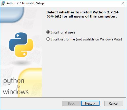
Windows does not come with Python, by default. Therefore, you will need to download/install it from python.org – get the latest 2.x version – currently https://www.python.org/downloads/release/python-2714/.
During the installation process, you will be asked if you want to install for all users or just yourself. That is up to you.
You’ll have the option of changing the default installation directory. We recommend keeping the default: C:\Python27.

Finally, you will have the choice of having this python executable be your default. That is up to you. If you have another Python distribution installed that you want to keep as your default, then you should leave this choice unchecked, i.e. leave the “X”. But if you do want to use this one as your default, select “Add python.exe to Path”:

After completing the Python 2.7 installation, open a Command Prompt shell and run (or if you selected to use this python.exe as your default in the above step, you can just use ‘python’ instead of specifying the full path):
c:\python27\python.exe -m pip install scipy
This will download and install the scipy module which is what our PhysiCell data reader uses. You can verify that it got installed by running python and trying to import it:
c:\>python27\python.exe
Python 2.7.14 (v2.7.14:84471935ed, Sep 16 2017, 20:25:58) [MSC v.1500 64 bit (AMD64)] on win32
Type "help", "copyright", "credits" or "license" for more information.
>>> import scipy
>>> quit()
OSX and Linux
Both OSX and Linux come with a system-level version of Python pre-installed (/usr/bin/python). Regardless of whether you have installed additional versions of Python, you will want to make sure the pre-installed version has the scipy module. OSX should already have it. However, Linux will not and you will need to install it via:
/usr/bin/python -m pip install scipy
You can test if scipy is accessible by simply trying to import it:
/usr/bin/python
...
>>> import scipy
>>> quit()
Installing ParaView
After you have successfully installed Python + scipy, download and install the (binary) ParaView application for your particular platform. The current, stable version is 5.4.1.
Windows
Assuming you have Admin permission, download/install ParaView-5.4.1-Qt5-OpenGL2-Windows-64bit.exe. If you do not have Admin permission, see Appendix A.
OSX or Linux
On OSX, assuming you have Admin permissions, download/install ParaView-5.4.1-Qt5-OpenGL2-MPI-OSX10.8-64bit.dmg. If you do not have Admin permission, see Appendix A.
On Linux, download ParaView-5.4.1-Qt5-OpenGL2-MPI-Linux-64bit.tar.gz and uncompress it into an appropriate directory. For example, if you want to make ParaView available to everyone, you may want to uncompress it into /usr/local. If you only want to make it available for your personal use, see Appendix A.
Running ParaView
Before starting the ParaView application, you can set an environment variable, PHYSICELL_DATA, to be the full path to the directory where the PhysiCell data can be found. This will make it easier for the custom data reader (a Python script) in the ParaView pipeline to find the data. For example, in the next section we provide a link to some sample PhysiCell data. If you simply uncompress that zip archive into your Downloads directory, then (on Linux/OSX bash) you could:
$ export PHYSICELL_DATA=/path-to-your-home-dir/Downloads
(this Windows tutorial, while aimed at editing your PATH, will also help you find the environment variables setting).
If you choose not to set the PHYSICELL_DATA environment variable, the custom data reader will look in your user Downloads directory. Alternatively, you can simply edit the ParaView custom data reader Python script to point to your data directory (and then you would probably want to File -> Save State).
NOTE: if you are using OSX and want to use the PHYSICELL_DATA environment variable, you should start the ParaView application from the Terminal, e.g. $ /Applications/ParaView-5.4.1.app/Contents/MacOS/paraview &
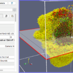
Finally, go ahead and start the ParaView application. You should see a blank GUI (Figure 1). Don’t be frightened by the complexity of the GUI – yes, there are several widgets, but we will walk you down a minimal path to help you visualize PhysiCell cell data. Of course you have access to all of ParaView’s documentation – the Getting Started, Guide, and Tutorial under the Help menu are a good place to start. In addition to the downloadable (.pdf) documentation, there is also in-depth information online: https://www.paraview.org/Wiki/ParaView
![]()
Figure 1. The ParaView application
Note: the 3-D axis in the lower-left corner of the RenderView does not represent the origin. It is just a reference axis to provide 3-D orientation.
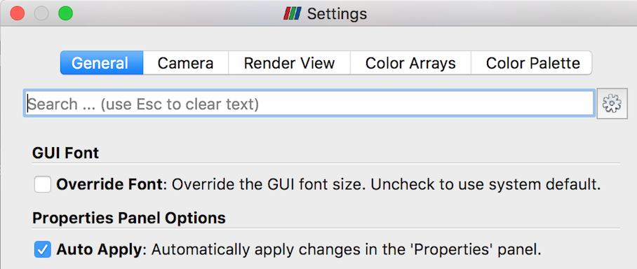
Before you get started with examples, you should open ParaView’s Settings (Preferences), select the General tab, and make sure “Auto Apply” is checked. This will avoid the need to manually “Apply” changes you make to an object’s properties.
Cancer immunity 3D example
We will use sample output data from the cancer_immune_3D project – one of the sample projects bundled with PhysiCell. You can refer to the PhysiCell Quickstart guide if you want to actually compile and run that project. But to simplify this tutorial, we provide sample data (a single time step) from that project, at:
https://sourceforge.net/projects/physicell/files/Tutorials/MultiCellDS/3D_PhysiCell_matlab_sample.zip/download
After you extract the files from this .zip, the file of interest for this tutorial is called output00003696_cells_physicell.mat. (And remember, as discussed above, to set the PHYSICELL_DATA environment variable to point to the directory where you extracted the files).
Additionally, for this tutorial, you’ll need some predefined ParaView state files (*.pvsm). A state file is just what it sounds like – it saves the entire state of a ParaView session so that you can easily re-use it. For this tutorial, we have provided the following state files to help you get started:
- physicell_glyphs.pvsm – render cells as simple vertex glyphs
- physicell_z0slice.pvsm – render the intersection of spherical glyphs with the Z=0 plane
- physicell_3clip_planes_ospray.pvsm – OSPRay renderer with 3 clipping planes
- physicell_cells_animate.pvsm – demonstrate how to do animation
Download them here: physicell_paraview_states.zip
Figure 2 is the SVG image from the sample data. It depicts the (3-D) cells that intersect the Z=0 plane.
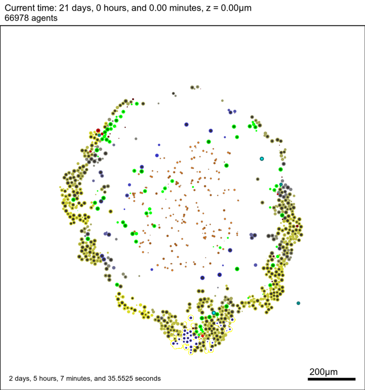
Figure 2. snapshot00003696.svg generated by PhysiCell
Reading PhysiCell (cell) data
One way that ParaView offers extensibility is via Python scripts. To make it easier to read data generated by PhysiCell, we provide users with a “Programmable Source” that will read and process data in a file. In the ParaView screen-captured figures below, the Programmable Source (“PhysiCellReader_cells”) will be the very first module in the pipeline.
For this exercise, you can File->LoadState and select the physicell_glyphs.pvsm file that you downloaded above. Assuming you previously copied the output00003696_cells_physicell.mat sample data file into one of the default directories as described above, it should display the results in Figure 3. (Otherwise, you will likely see an error message appear, in which case see Appendix B). These are the simplest (and fastest) glyphs to represent PhysiCell cells. They are known as 2-D Vertex glyphs, although the 2-D is misleading since they are rendered in 3-space. At this point, you can interact – rotate, zoom, pan, with the visualization (rf. Sect. 4.4.2 in the ParaViewGuide-5.4.0 for an explanation of the controls, but basically: left-mouse button hold while moving cursor to rotate; Ctl-left-mouse for zoom; Ctl-Shift-left-mouse to pan).
For this particular ParaView state file, we use the following code to assign colors to cells (Note: the PhysiCell code in /custom_modules creates the SVG file using colors based on cells’ neighbor information. This information is not saved in the .mat output files, therefore we cannot faithfully reproduce SVG cell colors here):
   # The following lines assign an integer to represent
   # a color, defined in a Color Map.
   sval = 0   # immune cells are yellow?
   if val[5,idx] == 1:  # [5]=cell_type
     sval = 1   # lime green
   if (val[6,idx] == 6) or (val[6,idx] == 7):
     sval = 0
   if val[7,idx] == 100:  # [7]=current_phase
     sval = 3   # apoptotic: red
   if val[7,idx] > 100 and val[7,idx] < 104:
     sval = 2   # necrotic: brownish
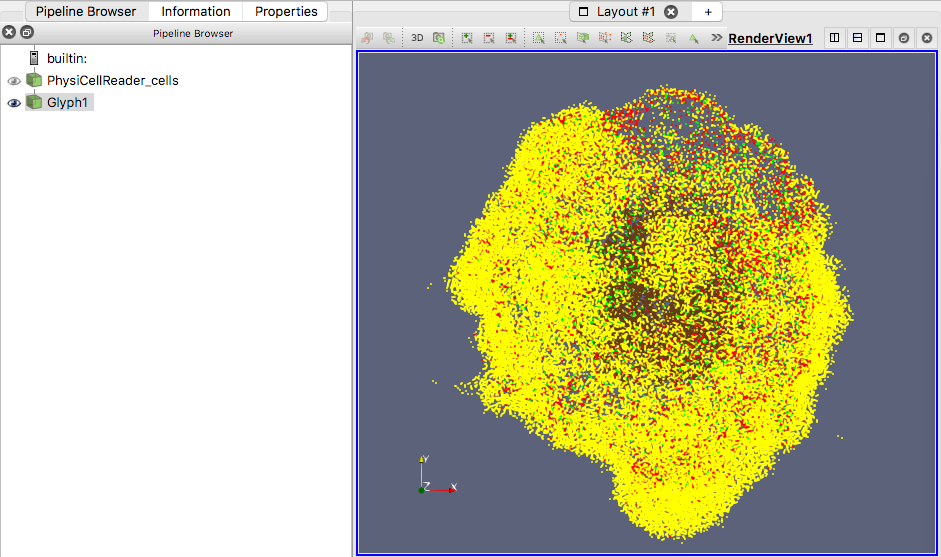
Figure 3. Glyphs as vertices

Figure 4. Glyphs as spheres
The next exercise is a simple extension of the previous. We want to add a slice to our pipeline that will intersect the cells (spherical glyphs). Assuming the slice is the Z=0 plane, this will approximate the SVG in Figure 2. So, select Edit->ResetSession to start from scratch, then File->LoadState and select the physicell_z0slice.pvsm file. Note that the “Glyph1” node in the pipeline is invisible (its “eyeball” is toggled off). If you make it visible (select the eyeball), you will essentially reproduce Figure 4. But for this exercise, we want Glyph1 to be invisible and Slice1 visible. If you select Slice1 (its green box) in the pipeline, you can select its Properties tab (at the top) to see all its properties. Of particular interest is the “Show Plane” checkbox at the top.
![]()
If this is checked on, you can interactively translate the plane along its normal, as well as select and rotate the normal itself. Try it! You can also “hardcode” the slice plane parameters in its properties panel.
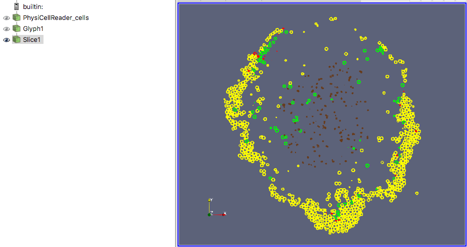
Figure 5. Z=0 slice through the spherical glyphs (approximate SVG slice)
Our final exercise with the sample dataset is to visualize cells using a higher quality renderer in ParaView known as OSPRay. So, as before, Edit->ResetSession to start from scratch, then File->LoadState and select the physicell_3clip_planes_ospray.pvsm file. This will create a pipeline that has 3 clipping planes aligned such that an octant of our spheroidal cell cluster is clipped away, letting us peer into its core (Figure 6). As with the previous slice plane, you can interactively reposition one or more of the clipping planes here.
Note: One (temporary) downside of using the OSPRay renderer is that cells (spheres) cannot be arbitrarily scaled in size. This will be fixed in a future release of ParaView. For now, we get around that by shrinking the distance of each cell from the origin. Obviously this is not a perfect solution, but for cells that are sort of clustered around the origin, it offers a decent approximation. We mention this 1) to disclose the inaccuracy, and 2) in case you look at the data ranges in the “Information” view/tab and notice they are not reflecting the domain of your simulation.
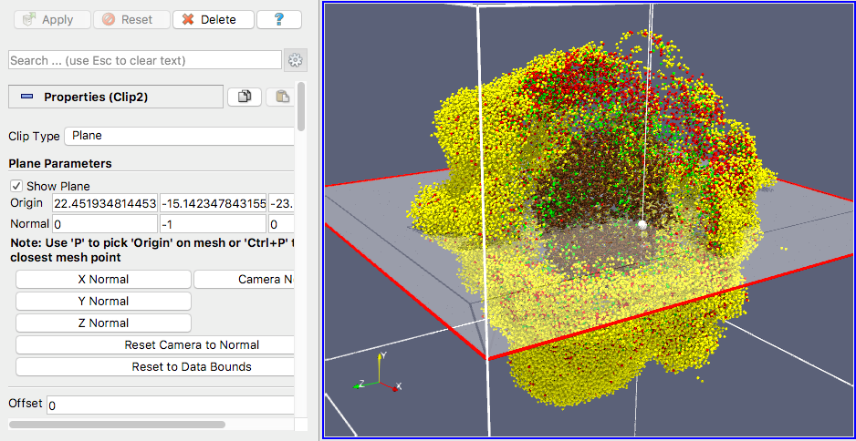
Figure 6. OSPRay-rendered cells, showing 1 of 3 interactive clipping planes
Animation in Time
At some point, you’ll want to see the dynamics of your simulation. This is where ParaView’s animation functionality comes in handy. It provides an easy way to let you render all (or a subset) of your PhysiCell output files, control the animation, and also save images (as .png files).
For this exercise, you will obviously want to have generated multiple output files from a PhysiCell project. Once you have those, e.g. from the cancer_immune_3D project, you can File->LoadState and select the physicell_cells_animate.pvsm file. This will show the following pipeline:

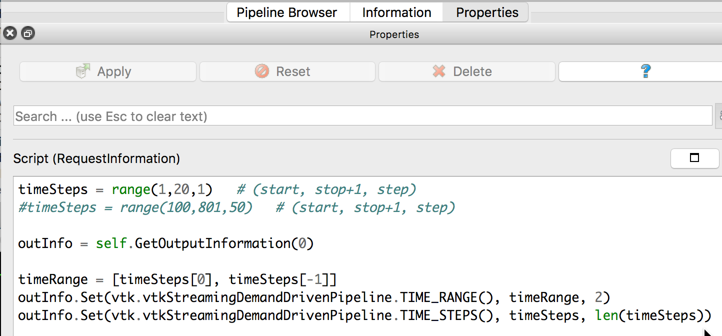
If you select the PhysiCellReader_cells (green box; leave its “eye” icon deselected) and click on the Properties tab, you will have access to the Script(RequestInformation) (you may need to click the “gear” icon next to the Properties tab Search bar to “Toggle advanced properties” to see this script):
In there, you will see the lines:
timeSteps = range(1,20,1)   # (start, stop+1, step)
#timeSteps = range(100,801,50)   # (start, stop+1 [, step])
You’ll want to edit the first line, specifying your desired start, stop, and (optionally) step values for your files’ numeric suffixes. We happened to use the second timeSteps line (currently commented out with the ‘#’) for data from our simulation, which resulted in 15 time steps (0-14) for the time values: 100,150,200,…800. Pressing the Play (center) button of the animation icons would animate those frames:
![]()
When you like what you see, you can select File->SaveAnimation to save the images. After you provide some minimal information for those images, e.g., resolution and filename prefix, press “OK” and you will see a horizontal progress bar being updated below the render window. After the animation images are generated, you can use your favorite image processing and movie generation tools to post-process them. In Figure 7, we used ImageMagick’s montage command to arrange the 15 images from a cancer_immune_3D simulation. And for generating a movie file, take a look at mplayer/mencoder as one open source option.
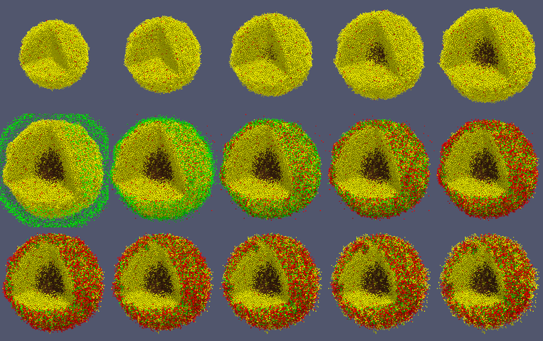
Figure 7. Images from cancer_immune_3D
Further Help
For questions specific to PhysiCell, have a look at our User Guide and join our mailing list to ask questions. For ParaView, have a look at their User Guide and join the ParaView mailing list to ask questions.
Thanks!
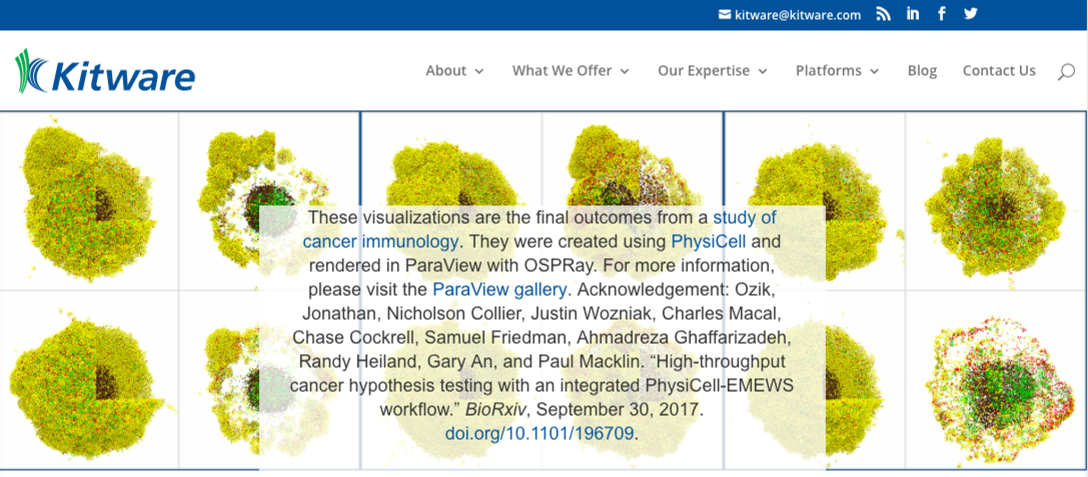
In closing, we would like to thank Kitware for their terrific open source software and the ParaView community (especially David DeMarle and Utkarsh Ayachit) for being so helpful answering questions and providing insight. We were honored that some of our early results got headlined on Kitware’s home page!
Appendix A: Installing without Admin permission
If you do not have Admin permission on your computer, we provide instructions for installing Python + scipy and ParaView using alternative approaches.
Windows
To install Python on Windows, without Admin permission, run the msiexec command on the .msi Python installer that you downloaded, specifying a (non-system) directory in which it should be installed via the targetdir keyword. After that completes, Python will be installed; however, the python command will not be in your PATH, i.e., it will not be globally accessible.
C:\Users\sue\Downloads>msiexec /a python-2.7.14.amd64.msi /qb targetdir=c:\py27

C:\Users\sue\Downloads>python
'python' is not recognized as an internal or external command,
operable program or batch file.

C:\Users\sue\Downloads>cd c:\py27

c:\py27>.\python.exe
Python 2.7.14 (v2.7.14:84471935ed, Sep 16 2017, 20:25:58) [MSC v.1500 64 bit (AMD64)] on win32
Type "help", "copyright", "credits" or "license" for more information.
>>>
Finally, download ParaView-5.4.1-Qt5-OpenGL2-Windows-64bit.zip and extract its contents into a permissible directory, e.g. under your home folder: C:\Users\sue\ParaView-5.4.1-Qt5-OpenGL2-Windows-64bit\
Then, in ParaView, using the Tools menu, open the Python Shell, and see if you can import scipy via:
>>> sys.path.insert(0,'c:\py27\Lib\site-packages')
>>> import scipy
Before proceeding with the tutorial using the PhysiCell state files, you will want to open ParaView’s Settings and check (toggle on) the “Auto Apply” property in the General settings tab.
OSX
OSX comes with a system Python pre-installed. And, at least with fairly recent versions of OSX, it comes with the scipy module also. You can test to see if that is the case on your system:
/usr/bin/python
>>> import scipy
To install ParaView, download a .pkg, not a .dmg, e.g. ParaView-5.4.1-Qt5-OpenGL2-MPI-OSX10.8-64bit.pkg. Then expand that .pkg contents into a permissible directory and untar its “Payload” which contains the actual paraview executable that you can open/run:
cd ~/Downloads
pkgutil --expand ParaView-5.4.1-Qt5-OpenGL2-MPI-OSX10.8-64bit.pkg ~/paraview
cd ~/paraview
tar -xvf Payload
open Contents/MacOS/paraview
Linux
Like OSX, Linux also comes with a system Python pre-installed. However, it does not come with the scipy module. To install the scipy Python module, run:
/usr/bin/python -m pip install scipy --user
To install and run ParaView, download the .tar.gz file, e.g. ParaView-5.4.1-Qt5-OpenGL2-MPI-Linux-64bit.tar.gz and uncompress it into a permissible directory. For example, from your home directory (after downloading):
mv ~/Downloads/ParaView-5.4.1-Qt5-OpenGL2-MPI-Linux-64bit.tar.gz .
tar -xvzf ParaView-5.4.1-Qt5-OpenGL2-MPI-Linux-64bit.tar.gz
cd ParaView-5.4.1-Qt5-OpenGL2-MPI-Linux-64bit/bin
./paraview
Appendix B: Editing the PhysiCellReader_cells Python Script
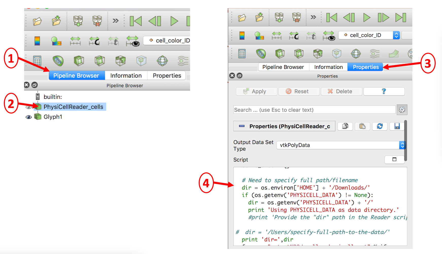
In case you encounter an error reading your .mat file(s) containing cell data, you will probably need to manually edit the directory path to the file. This is illustrated below in a 4-step process: 1) select the Pipeline Browser tab, 2) select the PhysiCellReader_cells object, 3) select its Properties, then 4) edit the relevant information in the (Python) script. (The script frame is scrollable).
Working with PhysiCell MultiCellDS digital snapshots in Matlab

PhysiCell 1.2.1 and later saves data as a specialized MultiCellDS digital snapshot, which includes chemical substrate fields, mesh information, and a readout of the cells and their phenotypes at single simulation time point. This tutorial will help you learn to use the matlab processing files included with PhysiCell.
This tutorial assumes you know (1) how to work at the shell / command line of your operating system, and (2) basic plotting and other functions in Matlab.
Key elements of a PhysiCell digital snapshot
A PhysiCell digital snapshot (a customized form of the MultiCellDS digital simulation snapshot) includes the following elements saved as XML and MAT files:
- output12345678.xml : This is the “base” output file, in MultiCellDS format. It includes key metadata such as when the file was created, the software, microenvironment information, and custom data saved at the simulation time. The Matlab files read this base file to find other related files (listed next). Example: output00003696.xml
- initial_mesh0.mat : This is the computational mesh information for BioFVM at time 0.0. Because BioFVM and PhysiCell do not use moving meshes, we do not save this data at any subsequent time.
- output12345678_microenvironment0.mat : This saves each biochemical substrate in the microenvironment at the computational voxels defined in the mesh (see above). Example: output00003696_microenvironment0.mat
- output12345678_cells.mat : This saves very basic cellular information related to BioFVM, including cell positions, volumes, secretion rates, uptake rates, and secretion saturation densities. Example: output00003696_cells.mat
- output12345678_cells_physicell.mat : This saves extra PhysiCell data for each cell agent, including volume information, cell cycle status, motility information, cell death information, basic mechanics, and any user-defined custom data. Example: output00003696_cells_physicell.mat
These snapshots make extensive use of Matlab Level 4 .mat files, for fast, compact, and well-supported saving of array data. Note that even if you cannot ready MultiCellDS XML files, you can work to parse the .mat files themselves.
The PhysiCell Matlab .m files
Every PhysiCell distribution includes some matlab functions to work with PhysiCell digital simulation snapshots, stored in the matlab subdirectory. The main ones are:
- composite_cutaway_plot.m : provides a quick, coarse 3-D cutaway plot of the discrete cells, with different colors for live (red), apoptotic (b), and necrotic (black) cells.
- read_MultiCellDS_xml.m : reads the “base” PhysiCell snapshot and its associated matlab files.
- set_MCDS_constants.m : creates a data structure MCDS_constants that has the same constants as PhysiCell_constants.h. This is useful for identifying cell cycle phases, etc.
- simple_cutaway_plot.m : provides a quick, coarse 3-D cutaway plot of user-specified cells.
- simple_plot.m : provides, a quick, coarse 3-D plot of the user-specified cells, without a cutaway or cross-sectional clipping plane.
A note on GNU Octave
Unfortunately, GNU octave does not include XML file parsing without some significant user tinkering. And one you’re done, it is approximately one order of magnitude slower than Matlab. Octave users can directly import the .mat files described above, but without the helpful metadata in the XML file. We’ll provide more information on the structure of these MAT files in a future blog post. Moreover, we plan to provide python and other tools for users without access to Matlab.
A sample digital snapshot
We provide a 3-D simulation snapshot from the final simulation time of the cancer-immune example in Ghaffarizadeh et al. (2017, in review) at:
The corresponding SVG cross-section for that time (through z = 0 μm) looks like this:

Unzip the sample dataset in any directory, and make sure the matlab files above are in the same directory (or in your Matlab path). If you’re inside matlab:
!unzip 3D_PhysiCell_matlab_sample.zip
Loading a PhysiCell MultiCellDS digital snapshot
Now, load the snapshot:
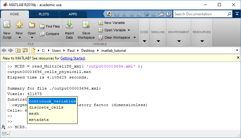
MCDS = read_MultiCellDS_xml( 'output00003696.xml');
This will load the mesh, substrates, and discrete cells into the MCDS data structure, and give a basic summary:
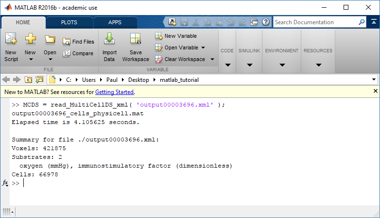
Typing ‘MCDS’ and then hitting ‘tab’ (for auto-completion) shows the overall structure of MCDS, stored as metadata, mesh, continuum variables, and discrete cells:
To get simulation metadata, such as the current simulation time, look at MCDS.metadata.current_time
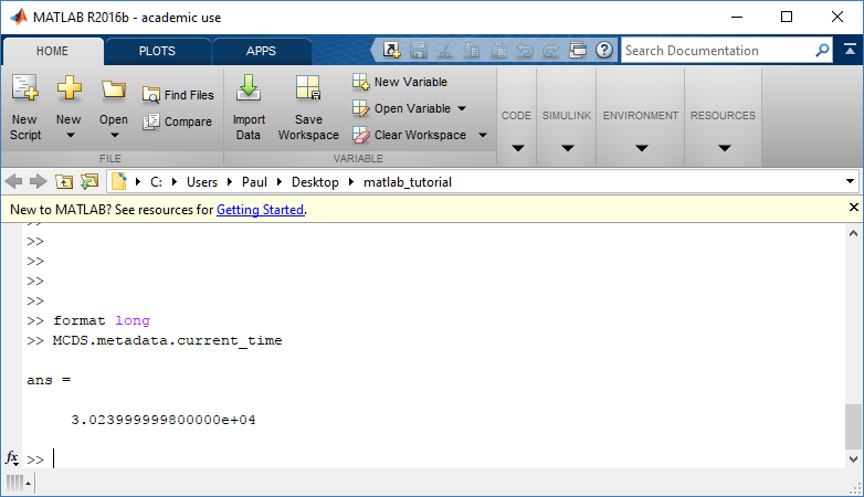
Here, we see that the current simulation time is 30240 minutes, or 21 days. MCDS.metadata.current_runtime gives the elapsed walltime to up to this point: about 53 hours (1.9e5 seconds), including file I/O time to write full simulation data once per 3 simulated minutes after the start of the adaptive immune response.
Plotting chemical substrates
Let’s make an oxygen contour plot through z = 0 μm. First, we find the index corresponding to this z-value:
k = find( MCDS.mesh.Z_coordinates == 0 );
Next, let’s figure out which variable is oxygen. Type “MCDS.continuum_variables.name”, which will show the array of variable names:
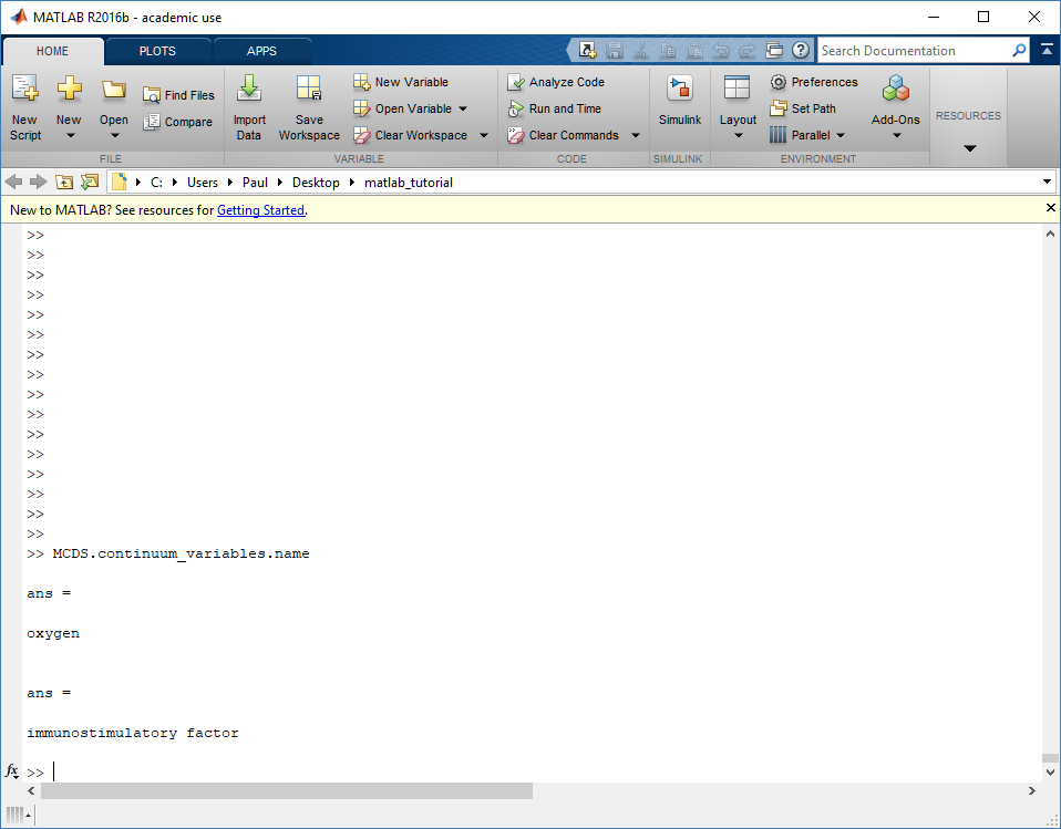
Here, oxygen is the first variable, (index 1). So, to make a filled contour plot:
contourf( MCDS.mesh.X(:,:,k), MCDS.mesh.Y(:,:,k), ...
     MCDS.continuum_variables(1).data(:,:,k) , 20 ) ;
Now, let’s set this to a correct aspect ratio (no stretching in x or y), add a colorbar, and set the axis labels, using
metadata to get labels:
axis image
colorbar
xlabel( sprintf( 'x (%s)' , MCDS.metadata.spatial_units) );
ylabel( sprintf( 'y (%s)' , MCDS.metadata.spatial_units) );
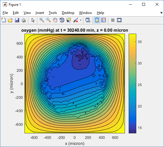
Lastly, let’s add an appropriate (time-based) title:
title( sprintf('%s (%s) at t = %3.2f %s, z = %3.2f %s', MCDS.continuum_variables(1).name , ...
     MCDS.continuum_variables(1).units , ...
     MCDS.metadata.current_time , ...
     MCDS.metadata.time_units, ...
     MCDS.mesh.Z_coordinates(k), ...
     MCDS.metadata.spatial_units ) );
Here’s the end result:
We can easily export graphics, such as to PNG format:
print( '-dpng' , 'output_o2.png' );
For more on plotting BioFVM data, see the tutorial
at http://www.mathcancer.org/blog/saving-multicellds-data-from-biofvm/
Plotting cells in space
3-D point cloud
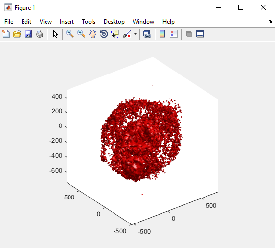
First, let’s plot all the cells in 3D:
plot3( MCDS.discrete_cells.state.position(:,1) , MCDS.discrete_cells.state.position(:,2), ...
	MCDS.discrete_cells.state.position(:,3) , 'bo' );
At first glance, this does not look good: some cells are far out of the simulation domain, distorting the automatic range of the plot:
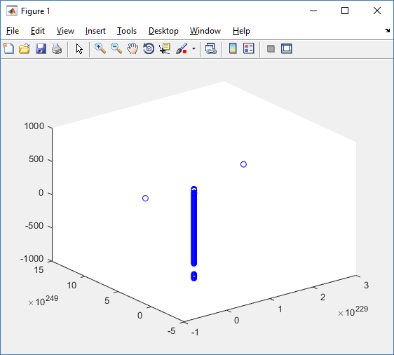
This does not ordinarily happen in PhysiCell (the default cell mechanics functions have checks to prevent such behavior), but this example includes a simple Hookean elastic adhesion model for immune cell attachment to tumor cells. In rare circumstances, an attached tumor cell or immune cell can apoptose on its own (due to its background apoptosis rate),
without “knowing” to detach itself from the surviving cell in the pair. The remaining cell attempts to calculate its elastic velocity based upon an invalid cell position (no longer in memory), creating an artificially large velocity that “flings” it out of the simulation domain. Such cells are not simulated any further, so this is effectively equivalent to an extra apoptosis event (only 3 cells are out of the simulation domain after tens of millions of cell-cell elastic adhesion calculations). Future versions of this example will include extra checks to prevent this rare behavior.
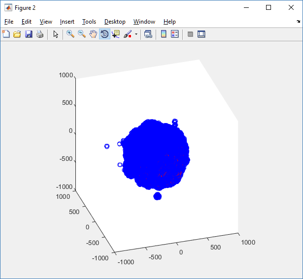
The plot can simply be fixed by changing the axis:
axis( 1000*[-1 1 -1 1 -1 1] )
axis square
Notice that this is a very difficult plot to read, and very non-interactive (laggy) to rotation and scaling operations. We can make a slightly nicer plot by searching for different cell types and plotting them with different colors:
% make it easier to work with the cell positions;
P = MCDS.discrete_cells.state.position;

% find type 1 cells
ind1 = find( MCDS.discrete_cells.metadata.type == 1 );
% better still, eliminate those out of the simulation domain
ind1 = find( MCDS.discrete_cells.metadata.type == 1 & ...
    abs(P(:,1))' < 1000 & abs(P(:,2))' < 1000 & abs(P(:,3))' < 1000 );

% find type 0 cells
ind0 = find( MCDS.discrete_cells.metadata.type == 0 & ...
    abs(P(:,1))' < 1000 & abs(P(:,2))' < 1000 & abs(P(:,3))' < 1000 );

%now plot them
P = MCDS.discrete_cells.state.position;
plot3( P(ind0,1), P(ind0,2), P(ind0,3), 'bo' )
hold on
plot3( P(ind1,1), P(ind1,2), P(ind1,3), 'ro' )
hold off
axis( 1000*[-1 1 -1 1 -1 1] )
axis square
However, this isn’t much better. You can use the scatter3 function to gain more control on the size and color of the plotted cells, or even make macros to plot spheres in the cell locations (with shading and lighting), but Matlab is very slow when plotting beyond 103 cells. Instead, we recommend the faster preview functions below for data exploration, and higher-quality plotting (e.g., by POV-ray) for final publication-
Fast 3-D cell data previewers
Notice that plot3 and scatter3 are painfully slow for any nontrivial number of cells. We can use a few fast previewers to quickly get a sense of the data. First, let’s plot all the dead cells, and make them red:
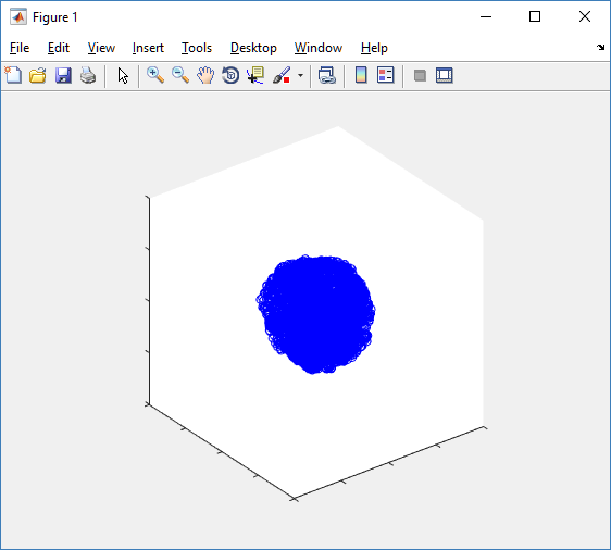
clf
simple_plot( MCDS,  MCDS, MCDS.discrete_cells.dead_cells , 'r' )
This function creates a coarse-grained 3-D indicator function (0 if no cells are present; 1 if they are), and plots a 3-D level surface. It is very responsive to rotations and other operations to explore the data. You may notice the second argument is a list of indices: only these cells are plotted. This gives you a method to select cells with specific characteristics when plotting. (More on that below.) If you want to get a sense of the interior structure, use a cutaway plot:
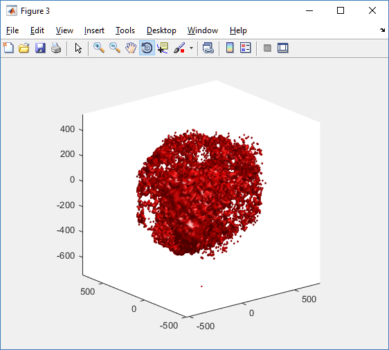
clf
simple_cutaway_plot( MCDS, MCDS, MCDS.discrete_cells.dead_cells , 'r' )
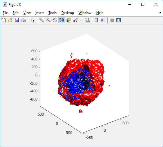
We also provide a fast “composite” cutaway which plots all live cells as red, apoptotic cells as blue (without the cutaway), and all necrotic cells as black:
clf
composite_cutaway_plot( MCDS )
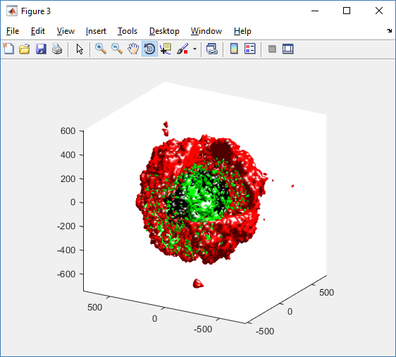
Lastly, we show an improved plot that uses different colors for the immune cells, and Matlab’s “find” function to help set up the indexing:
constants = set_MCDS_constants

% find the type 0 necrotic cells
ind0_necrotic = find( MCDS.discrete_cells.metadata.type == 0 & ...
    (MCDS.discrete_cells.phenotype.cycle.current_phase == constants.necrotic_swelling | ...
    MCDS.discrete_cells.phenotype.cycle.current_phase == constants.necrotic_lysed | ...
    MCDS.discrete_cells.phenotype.cycle.current_phase == constants.necrotic) );

% find the live type 0 cells
ind0_live = find( MCDS.discrete_cells.metadata.type == 0 & ...
    (MCDS.discrete_cells.phenotype.cycle.current_phase ~= constants.necrotic_swelling & ...
    MCDS.discrete_cells.phenotype.cycle.current_phase ~= constants.necrotic_lysed & ...
    MCDS.discrete_cells.phenotype.cycle.current_phase ~= constants.necrotic & ...
    MCDS.discrete_cells.phenotype.cycle.current_phase ~= constants.apoptotic) );

clf
% plot live tumor cells red, in cutaway view
simple_cutaway_plot( MCDS, ind0_live , 'r' );
hold on
% plot dead tumor cells black, in cutaway view
simple_cutaway_plot( MCDS, ind0_necrotic , 'k' )
% plot all immune cells, but without cutaway (to show how they infiltrate)
simple_plot( MCDS, ind1, 'g' )
hold off
A small cautionary note on future compatibility
PhysiCell 1.2.1 uses the <custom> data tag (allowed as part of the MultiCellDS specification) to encode its cell data, to allow a more compact data representation, because the current PhysiCell daft does not support such a formulation, and Matlab is painfully slow at parsing XML files larger than ~50 MB. Thus, PhysiCell snapshots are not yet fully compatible with general MultiCellDS tools, which would by default ignore custom data. In the future, we will make available converter utilities to transform “native” custom PhysiCell snapshots to MultiCellDS snapshots that encode all the cellular information in a more verbose but compatible XML format.
Closing words and future work
Because Octave is not a great option for parsing XML files (with critical MultiCellDS metadata), we plan to write similar functions to read and plot PhysiCell snapshots in Python, as an open source alternative. Moreover, our lab in the next year will focus on creating further MultiCellDS configuration, analysis, and visualization routines. We also plan to provide additional 3-D functions for plotting the discrete cells and varying color with their properties.
In the longer term, we will develop open source, stand-alone analysis and visualization tools for MultiCellDS snapshots (including PhysiCell snapshots). Please stay tuned!
Saving MultiCellDS data from BioFVM
Note: This is part of a series of “how-to” blog posts to help new users and developers of BioFVM.
Introduction
A major initiative for my lab has been MultiCellDS: a standard for multicellular data. The project aims to create model-neutral representations of simulation data (for both discrete and continuum models), which can also work for segmented experimental and clinical data. A single-time output is called a digital snapshot. An interdisciplinary, multi-institutional review panel has been hard at work to nail down the draft standard.
A BioFVM MultiCellDS digital snapshot includes program and user metadata (more information to be included in a forthcoming publication), an output of the microenvironment, and any cells that are secreting or uptaking substrates.
As of Version 1.1.0, BioFVM supports output saved to MultiCellDS XML files. Each download also includes a matlab function for importing MultiCellDS snapshots saved by BioFVM programs. This tutorial will get you going.
BioFVM (finite volume method for biological problems) is an open source code for solving 3-D diffusion of 1 or more substrates. It was recently published as open access in Bioinformatics here:
http://dx.doi.org/10.1093/bioinformatics/btv730
The project website is at http://BioFVM.MathCancer.org, and downloads are at http://BioFVM.sf.net.
Working with MultiCellDS in BioFVM programs
We include a MultiCellDS_test.cpp file in the examples directory of every BioFVM download (Version 1.1.0 or later). Create a new project directory, copy the following files to it:
- BioFVM*.cpp and BioFVM*.h (from the main BioFVM directory)
- pugixml.* (from the main BioFVM directory)
- Makefile and MultiCellDS_test.cpp (from the examples directory)
Open the MultiCellDS_test.cpp file to see the syntax as you read the rest of this post.
See earlier tutorials (below) if you have troubles with this.
Setting metadata values
There are few key bits of metadata. First, the program used for the simulation (all these fields are optional):
// the program name, version, and project website:
BioFVM_metadata.program.program_name = "BioFVM MultiCellDS Test";
BioFVM_metadata.program.program_version = "1.0";
BioFVM_metadata.program.program_URL = "http://BioFVM.MathCancer.org";

// who created the program (if known)
BioFVM_metadata.program.creator.surname = "Macklin";
BioFVM_metadata.program.creator.given_names = "Paul";
BioFVM_metadata.program.creator.email = "Paul.Macklin@usc.edu";
BioFVM_metadata.program.creator.URL = "http://BioFVM.MathCancer.org";
BioFVM_metadata.program.creator.organization = "University of Southern California";
BioFVM_metadata.program.creator.department = "Center for Applied Molecular Medicine";
BioFVM_metadata.program.creator.ORCID = "0000-0002-9925-0151";

// (generally peer-reviewed) citation information for the program
BioFVM_metadata.program.citation.DOI = "10.1093/bioinformatics/btv730";
BioFVM_metadata.program.citation.PMID = "26656933";
BioFVM_metadata.program.citation.PMCID = "PMC1234567";
BioFVM_metadata.program.citation.text = "A. Ghaffarizadeh, S.H. Friedman, and P. Macklin,
    BioFVM: an efficient parallelized diffusive transport solver for 3-D biological
    simulations, Bioinformatics, 2015. DOI: 10.1093/bioinformatics/btv730.";
BioFVM_metadata.program.citation.notes = "notes here";
BioFVM_metadata.program.citation.URL = "http://dx.doi.org/10.1093/bioinformatics/btv730";

// user information: who ran the program
BioFVM_metadata.program.user.surname = "Kirk";
BioFVM_metadata.program.user.given_names = "James T.";
BioFVM_metadata.program.user.email = "Jimmy.Kirk@starfleet.mil";
BioFVM_metadata.program.user.organization = "Starfleet";
BioFVM_metadata.program.user.department = "U.S.S. Enterprise (NCC 1701)";
BioFVM_metadata.program.user.ORCID = "0000-0000-0000-0000";

// And finally, data citation information (the publication where this simulation snapshot appeared)
BioFVM_metadata.data_citation.DOI = "10.1093/bioinformatics/btv730";
BioFVM_metadata.data_citation.PMID = "12345678";
BioFVM_metadata.data_citation.PMCID = "PMC1234567";
BioFVM_metadata.data_citation.text = "A. Ghaffarizadeh, S.H. Friedman, and P. Macklin, BioFVM:
    an efficient parallelized diffusive transport solver for 3-D biological simulations, Bioinformatics,
    2015. DOI: 10.1093/bioinformatics/btv730.";
BioFVM_metadata.data_citation.notes = "notes here";
BioFVM_metadata.data_citation.URL = "http://dx.doi.org/10.1093/bioinformatics/btv730";
You can sync the metadata current time, program runtime (wall time), and dimensional units using the following command. (This command is automatically run whenever you use the save command below.)
BioFVM_metadata.sync_to_microenvironment( M );
You can display a basic summary of the metadata via:
BioFVM_metadata.display_information( std::cout );
Setting options
By default (to save time and disk space), BioFVM saves the mesh as a Level 3 matlab file, whose location is embedded into the MultiCellDS XML file. You can disable this feature and revert to full XML (e.g., for human-readable cross-model reporting) via:
set_save_biofvm_mesh_as_matlab( false );
Similarly, BioFVM defaults to saving the values of the substrates in a compact Level 3 matlab file. You can override this with:
set_save_biofvm_data_as_matlab( false );
BioFVM by default saves the cell-centered sources and sinks. These take a lot of time to parse because they require very hierarchical data structures. You can disable saving the cells (basic_agents) via:
set_save_biofvm_cell_data( false );
Lastly, when you do save the cells, we default to a customized, minimal matlab format. You can revert to a more standard (but much larger) XML format with:
set_save_biofvm_cell_data_as_custom_matlab( false )
Saving a file
Saving the data is very straightforward:
save_BioFVM_to_MultiCellDS_xml_pugi( "sample" , M , current_simulation_time );
Your data will be saved in sample.xml. (Depending upon your options, it may generate several .mat files beginning with “sample”.)
If you’d like the filename to depend upon the simulation time, use something more like this:
double current_simulation_time = 10.347;
char filename_base [1024];
sprintf( &filename_base , "sample_%f", current_simulation_time );
save_BioFVM_to_MultiCellDS_xml_pugi( filename_base , M,
   current_simulation_time );
Your data will be saved in sample_10.347000.xml. (Depending upon your options, it may generate several .mat files beginning with “sample_10.347000”.)
Compiling and running the program:
Edit the Makefile as below:
PROGRAM_NAME := MCDS_test

all: $(BioFVM_OBJECTS) $(pugixml_OBJECTS) MultiCellDS_test.cpp

$(COMPILE_COMMAND) -o $(PROGRAM_NAME) $(BioFVM_OBJECTS) $(pugixml_OBJECTS) MultiCellDS_test.cpp
If you’re running OSX, you’ll probably need to update the compiler from “g++”. See these tutorials.
Then, at the command prompt:
make
./MCDS_test
On Windows, you’ll need to run without the ./:
make
MCDS_test
Working with MultiCellDS data in Matlab
Reading data in Matlab
Copy the read_MultiCellDS_xml.m file from the matlab directory (included in every MultiCellDS download). To read the data, just do this:
MCDS = read_MultiCellDS_xml( 'sample.xml' );
This should take around 30 seconds for larger data files (500,000 to 1,000,000 voxels with a few substrates, and around 250,000 cells). The long execution time is primarily because Matlab is ghastly inefficient at loops over hierarchical data structures. Increasing to 1,000,000 cells requires around 80-90 seconds to parse in matlab.
Plotting data in Matlab
Plotting the 3-D substrate data
First, let’s do some basic contour and surface plotting:
mid_index = round( length(MCDS.mesh.Z_coordinates)/2 );

contourf( MCDS.mesh.X(:,:,mid_index), ...
	MCDS.mesh.Y(:,:,mid_index), ...
	MCDS.continuum_variables(2).data(:,:,mid_index) , 20 ) ;
axis image
colorbar
xlabel( sprintf( 'x (%s)' , MCDS.metadata.spatial_units) );
ylabel( sprintf( 'y (%s)' , MCDS.metadata.spatial_units) );
title( sprintf('%s (%s) at t = %f %s, z = %f %s', MCDS.continuum_variables(2).name , ...
	MCDS.continuum_variables(2).units , ...
	MCDS.metadata.current_time , ...
	MCDS.metadata.time_units, ...
	MCDS.mesh.Z_coordinates(mid_index), ...
	MCDS.metadata.spatial_units ) );
OR
contourf( MCDS.mesh.X_coordinates , MCDS.mesh.Y_coordinates, ...
	MCDS.continuum_variables(2).data(:,:,mid_index) , 20 ) ;
axis image
colorbar
xlabel( sprintf( 'x (%s)' , MCDS.metadata.spatial_units) );
ylabel( sprintf( 'y (%s)' , MCDS.metadata.spatial_units) );
title( sprintf('%s (%s) at t = %f %s, z = %f %s', ...
	MCDS.continuum_variables(2).name , ...
	MCDS.continuum_variables(2).units , ...
	MCDS.metadata.current_time , ...
	MCDS.metadata.time_units, ...
	MCDS.mesh.Z_coordinates(mid_index), ...
	MCDS.metadata.spatial_units ) );
Here’s a surface plot:
surf( MCDS.mesh.X_coordinates , MCDS.mesh.Y_coordinates, ...
	MCDS.continuum_variables(1).data(:,:,mid_index) ) ;
colorbar
axis tight
xlabel( sprintf( 'x (%s)' , MCDS.metadata.spatial_units) );
ylabel( sprintf( 'y (%s)' , MCDS.metadata.spatial_units) );
zlabel( sprintf( '%s (%s)', MCDS.continuum_variables(1).name, ...
	MCDS.continuum_variables(1).units ) );
title( sprintf('%s (%s) at t = %f %s, z = %f %s', MCDS.continuum_variables(1).name , ...
	MCDS.continuum_variables(1).units , ...
	MCDS.metadata.current_time , ...
	MCDS.metadata.time_units, ...
	MCDS.mesh.Z_coordinates(mid_index), ...
	MCDS.metadata.spatial_units ) );
Finally, here are some more advanced plots. The first is an “exploded” stack of contour plots:
clf
contourslice( MCDS.mesh.X , MCDS.mesh.Y, MCDS.mesh.Z , ...
	MCDS.continuum_variables(2).data , [],[], ...
	MCDS.mesh.Z_coordinates(1:15:length(MCDS.mesh.Z_coordinates)),20);
view([-45 10]);
axis tight;
xlabel( sprintf( 'x (%s)' , MCDS.metadata.spatial_units) );
ylabel( sprintf( 'y (%s)' , MCDS.metadata.spatial_units) );
zlabel( sprintf( 'z (%s)' , MCDS.metadata.spatial_units) );
title( sprintf('%s (%s) at t = %f %s', ...
	MCDS.continuum_variables(2).name , ...
	MCDS.continuum_variables(2).units , ...
	MCDS.metadata.current_time, ...
	MCDS.metadata.time_units ) );
Next, we show how to use isosurfaces with transparency
clf
patch( isosurface( MCDS.mesh.X , MCDS.mesh.Y, MCDS.mesh.Z, ...
	MCDS.continuum_variables(1).data, 1000 ), 'edgecolor', ...
	'none', 'facecolor', 'r' , 'facealpha' , 1 );
hold on
patch( isosurface( MCDS.mesh.X , MCDS.mesh.Y, MCDS.mesh.Z, ...
MCDS.continuum_variables(1).data, 5000 ), 'edgecolor', ...
	'none', 'facecolor', 'b' , 'facealpha' , 0.7 );
patch( isosurface( MCDS.mesh.X , MCDS.mesh.Y, MCDS.mesh.Z, ...
	MCDS.continuum_variables(1).data, 10000 ), 'edgecolor', ...
	'none', 'facecolor', 'g' , 'facealpha' , 0.5 );
hold off
% shading interp
camlight
view(3)
axis image
axis tightcamlight lighting gouraud
xlabel( sprintf( 'x (%s)' , MCDS.metadata.spatial_units) );
ylabel( sprintf( 'y (%s)' , MCDS.metadata.spatial_units) );
zlabel( sprintf( 'z (%s)' , MCDS.metadata.spatial_units) );
title( sprintf('%s (%s) at t = %f %s', ...
	MCDS.continuum_variables(1).name , ...
	MCDS.continuum_variables(1).units , ...
	MCDS.metadata.current_time, ...
	MCDS.metadata.time_units ) );
You can get more 3-D volumetric visualization ideas at Matlab’s website. This visualization post at MIT also has some great tips.
Plotting the cells
Here is a basic 3-D plot for the cells:
plot3( MCDS.discrete_cells.state.position(:,1) , ...
	MCDS.discrete_cells.state.position(:,2) , ...
	MCDS.discrete_cells.state.position(:,3) , 'bo' );
view(3)
axis tight
xlabel( sprintf( 'x (%s)' , MCDS.metadata.spatial_units) );
ylabel( sprintf( 'y (%s)' , MCDS.metadata.spatial_units) );
zlabel( sprintf( 'z (%s)' , MCDS.metadata.spatial_units) );
title( sprintf('Cells at t = %f %s', MCDS.metadata.current_time, ...
	MCDS.metadata.time_units ) );
plot3 is more efficient than scatter3, but scatter3 will give more coloring options. Here is the syntax:
scatter3( MCDS.discrete_cells.state.position(:,1), ...
	MCDS.discrete_cells.state.position(:,2), ...
	MCDS.discrete_cells.state.position(:,3) , 'bo' );
view(3)
axis tight
xlabel( sprintf( 'x (%s)' , MCDS.metadata.spatial_units) );
ylabel( sprintf( 'y (%s)' , MCDS.metadata.spatial_units) );
zlabel( sprintf( 'z (%s)' , MCDS.metadata.spatial_units) );
title( sprintf('Cells at t = %f %s', MCDS.metadata.current_time, ...
	MCDS.metadata.time_units ) );
Jan Poleszczuk gives some great insights on plotting many cells in 3D at his blog. I’d recommend checking out his post on visualizing a cellular automaton model. At some point, I’ll update this post with prettier plotting based on his methods.
What’s next
Future releases of BioFVM will support reading MultiCellDS snapshots (for model initialization).
Matlab is pretty slow at parsing and visualizing large amounts of data. We also plan to include resources for accessing MultiCellDS data in VTK / Paraview and Python.
Return to News • Return to MathCancer • Follow @MathCancer