Category: Uncategorized
Introducing cell interactions & transformations
Introduction
PhysiCell 1.10.0 introduces a number of new features designed to simplify modeling of complex interactions and transformations. This blog post will introduce the underlying mathematics and show a complete example. We will teach this and other examples in greater depth at our upcoming Virtual PhysiCell Workshop & Hackathon (July 24-30, 2022). (Apply here!!)
Cell Interactions
In the past, it has been possible to model complex cell-cell interactions (such as those needed for microecology and immunology) by connecting basic cell functions for interaction testing and custom functions. In particular, these functions were used for the COVID19 Coalition’s open source model of SARS-CoV-2 infections and immune responses. We now build upon that work to standardize and simplify these processes, making use of the cell’s state.neighbors (a list of all cells deemed to be within mechanical interaction distance).
All the parameters for cell-cell interactions are stored in cell.phenotype.cell_interactions.
Phagocytosis
A cell can phagocytose (ingest) another cell, with rates that vary with the cell’s live/dead status or the cell type. In particular, we store:
- double dead_phagocytosis_rate : This is the rate at which a cell can phagocytose a dead cell of any type.
std::vector<double> live_phagocytosis_rates: This is a vector of phagocytosis rates for live cells of specific types. If there are n cell definitions in the simulation, then there are n rates in this vector. Please note that the index i for any cell type is its index in the list of cell definitions, not necessarily the ID of its cell definition. For safety, use one of the following to determine that index:find_cell_definition_index( int type_ID ): search for the cell definition’s index by its type ID (cell.type)find_cell_definition_index( std::string type_name ): search for the cell definition’s index by its human-readable type name (cell.type_name)
We also supply a function to help access these live phagocytosis rates.
- double& live_phagocytosis_rate( std::string type_name ) : Directly access the cell’s rate of phagocytosing the live cell type by its human-readable name. For example,
pCell->phenotype.cell_interactions.live_phagocytosis_rate( "tumor cell" ) = 0.01;
At each mechanics time step (with duration \(\Delta t\), default 0.1 minutes), each cell runs through its list of neighbors. If the neighbor is dead, its probability of phagocytosing it between \(t\) and \(t+\Delta t\) is
\[ \verb+dead_phagocytosis_rate+ \cdot \Delta t\]
If the neighbor cell is alive and its type has index j, then its probability of phagocytosing the cell between \(t\) and \(t+\Delta t\) is
\[ \verb+live_phagocytosis_rates[j]+ \cdot \Delta t\]
PhysiCell’s standardized phagocytosis model does the following:
- The phagocytosing cell will absorb the phagocytosed cell’s total solid volume into the cytoplasmic solid volume
- The phagocytosing cell will absorb the phagocytosed cell’s total fluid volume into the fluid volume
- The phagocytosing cell will absorb all of the phagocytosed cell’s internalized substrates.
- The phagocytosed cell is set to zero volume, flagged for removal, and set to not mechanically interact with remaining cells.
- The phagocytosing cell does not change its target volume. The standard volume model will gradually “digest” the absorbed volume as the cell shrinks towards its target volume.
Cell Attack
A cell can attack (cause damage to) another live cell, with rates that vary with the cell’s type. In particular, we store:
- double damage_rate : This is the rate at which a cell causes (dimensionless) damage to a target cell. The cell’s total damage is stored in cell.state.damage. The total integrated attack time is stored in
cell.state.total_attack_time. std::vector<double> attack_rates: This is a vector of attack rates for live cells of specific types. If there are n cell definitions in the simulation, then there are n rates in this vector. Please note that the index i for any cell type is its index in the list of cell definitions, not necessarily the ID of its cell definition. For safety, use one of the following to determine that index:find_cell_definition_index( int type_ID ): search for the cell definition’s index by its type ID (cell.type)find_cell_definition_index( std::string type_name ): search for the cell definition’s index by its human-readable type name (cell.type_name)
We also supply a function to help access these attack rates.
- double& attack_rate( std::string type_name ) : Directly access the cell’s rate of attacking the live cell type by its human-readable name. For example,
pCell->phenotype.cell_interactions.attack_rate( "tumor cell" ) = 0.01;
At each mechanics time step (with duration \(\Delta t\), default 0.1 minutes), each cell runs through its list of neighbors. If the neighbor cell is alive and its type has index j, then its probability of attacking the cell between \(t\) and \(t+\Delta t\) is
\[ \verb+attack_rates[j]+ \cdot \Delta t\]
To attack the cell:
- The attacking cell will increase the target cell’s damage by \( \verb+damage_rate+ \cdot \Delta t\).
- The attacking cell will increase the target cell’s total attack time by \(\Delta t\).
Note that this allows us to have variable rates of damage (e.g., some immune cells may be “worn out”), and it allows us to distinguish between damage and integrated interaction time. (For example, you may want to write a model where damage can be repaired over time.)
As of this time, PhysiCell does not have a standardized model of death in response to damage. It is up to the modeler to vary a death rate with the total attack time or integrated damage, based on their hypotheses. For example:
\[ r_\textrm{apoptosis} = r_\textrm{apoptosis,0} + \left( r_\textrm{apoptosis,max} – r_\textrm{apoptosis,0} \right) \cdot \frac{ d^h }{ d_\textrm{halfmax}^h + d^h } \]
In a phenotype function, we might write this as:
void damage_response( Cell* pCell, Phenotype& phenotype, double dt )
{ // get the base apoptosis rate from our cell definition
     Cell_Definition* pCD = find_cell_definition( pCell->type_name );
     double apoptosis_0 = pCD->phenotype.death.rates[0];
     double apoptosis_max = 100 * apoptosis_0;
     double half_max = 2.0;
     double damage = pCell->state.damage;
     phenotype.death.rates[0] = apoptosis_0 +
(apoptosis_max -apoptosis_0) * Hill_response_function(d,half_max,1.0);
     return;
}
Cell Fusion
A cell can fuse with another live cell, with rates that vary with the cell’s type. In particular, we store:
std::vector<double> fusion_rates: This is a vector of fusion rates for live cells of specific types. If there are n cell definitions in the simulation, then there are n rates in this vector. Please note that the index i for any cell type is its index in the list of cell definitions, not necessarily the ID of its cell definition. For safety, use one of the following to determine that index:find_cell_definition_index( int type_ID ): search for the cell definition’s index by its type ID (cell.type)find_cell_definition_index( std::string type_name ): search for the cell definition’s index by its human-readable type name (cell.type_name)
We also supply a function to help access these fusion rates.
- double& fusion_rate( std::string type_name ) : Directly access the cell’s rate of fusing with the live cell type by its human-readable name. For example,
pCell->phenotype.cell_interactions.fusion_rate( "tumor cell" ) = 0.01;
At each mechanics time step (with duration \(\Delta t\), default 0.1 minutes), each cell runs through its list of neighbors. If the neighbor cell is alive and its type has index j, then its probability of fusing with the cell between \(t\) and \(t+\Delta t\) is
\[ \verb+fusion_rates[j]+ \cdot \Delta t\]
PhysiCell’s standardized fusion model does the following:
- The fusing cell will absorb the fused cell’s total cytoplasmic solid volume into the cytoplasmic solid volume
- The fusing cell will absorb the fused cell’s total nuclear volume into the nuclear solid volume
- The fusing cell will keep track of its number of nuclei in
state.number_of_nuclei. (So, if the fusing cell has 3 nuclei and the fused cell has 2 nuclei, then the new cell will have 5 nuclei.) - The fusing cell will absorb the fused cell’s total fluid volume into the fluid volume
- The fusing cell will absorb all of the fused cell’s internalized substrates.
- The fused cell is set to zero volume, flagged for removal, and set to not mechanically interact with remaining cells.
- The fused cell will be moved to the (volume weighted) center of mass of the two original cells.
- The fused cell does change its target volume to the sum of the original two cells’ target volumes. The combined cell will grow / shrink towards its new target volume.
Cell Transformations
A live cell can transform to another type (e.g., via differentiation). We store parameters for cell transformations in cell.phenotype.cell_transformations, particularly:
std::vector<double> transformation_rates: This is a vector of transformation rates from a cell’s current to type to one of the other cell types. If there are n cell definitions in the simulation, then there are n rates in this vector. Please note that the index i for any cell type is its index in the list of cell definitions, not necessarily the ID of its cell definition. For safety, use one of the following to determine that index:find_cell_definition_index( int type_ID ): search for the cell definition’s index by its type ID (cell.type)find_cell_definition_index( std::string type_name ): search for the cell definition’s index by its human-readable type name (cell.type_name)
We also supply a function to help access these transformation rates.
- double& transformation_rate( std::string type_name ) : Directly access the cell’s rate of transforming into a specific cell type by searching for its human-readable name. For example,
pCell->phenotype.cell_transformations.transformation_rate( "mutant tumor cell" ) = 0.01;
At each phenotype time step (with duration \(\Delta t\), default 6 minutes), each cell runs through the vector of transformation rates. If a (different) cell type has index j, then the cell’s probability transforming to that type between \(t\) and \(t+\Delta t\) is
\[ \verb+transformation_rates[j]+ \cdot \Delta t\]
PhysiCell uses the built-in Cell::convert_to_cell_definition( Cell_Definition& ) for the transformation.
Other New Features
This release also includes a number of handy new features:
Advanced Chemotaxis
After setting chemotaxis sensitivities in phenotype.motility and enabling the feature, cells can chemotax based on linear combinations of substrate gradients.
std::vector<double> phenotype.motility.chemotactic_sensitivitiesis a vector of chemotactic sensitivities, one for each substrate in the environment. By default, these are all zero for backwards compatibility. A positive sensitivity denotes chemotaxis up a corresponding substrate’s gradient (towards higher values), whereas a negative sensitivity gives chemotaxis against a gradient (towards lower values).- For convenience, you can access (read and write) a substrate’s chemotactic sensitivity via
phenotype.motility.chemotactic_sensitivity(name)wherenameis the human-readable name of a substrate in the simulation. - If the user sets
cell.cell_functions.update_migration_bias = advanced_chemotaxis_function, then these sensitivities are used to set the migration bias direction via: \[\vec{d}_\textrm{mot} = s_0 \nabla \rho_0 + \cdots + s_n \nabla \rho_n. \] - If the user sets
cell.cell_functions.update_migration_bias = advanced_chemotaxis_function_normalized, then these sensitivities are used to set the migration bias direction via: \[\vec{d}_\textrm{mot} = s_0 \frac{\nabla\rho_0}{|\nabla\rho_0|} + \cdots + s_n \frac{ \nabla \rho_n }{|\nabla\rho_n|}.\]
Cell Adhesion Affinities
cell.phenotype.mechanics.adhesion_affinitiesis a vector of adhesive affinities, one for each cell type in the simulation. By default, these are all one for backwards compatibility.- For convenience, you can access (read and write) a cell’s adhesive affinity for a specific cell type via
phenotype.mechanics.adhesive_affinity(name), wherenameis the human-readable name of a cell type in the simulation. - The standard mechanics function (based on potentials) uses this as follows. If cell
ihas an cell-cell adhesion strengtha_iand an adhesive affinityp_ijto cell typej, and if celljhas a cell-cell adhesion strength ofa_jand an adhesive affinityp_jito cell typei, then the strength of their adhesion is \[ \sqrt{ a_i p_{ij} \cdot a_j p_{ji} }.\] Notice that if \(a_i = a_j\) and \(p_{ij} = p_{ji}\), then this reduces to \(a_i a_{pj}\). - The standard elastic spring function (
standard_elastic_contact_function) uses this as follows. If cellihas an elastic constanta_iand an adhesive affinityp_ijto cell typej, and if celljhas an elastic constanta_jand an adhesive affinityp_jito cell typei, then the strength of their adhesion is \[ \sqrt{ a_i p_{ij} \cdot a_j p_{ji} }.\] Notice that if \(a_i = a_j\) and \(p_{ij} = p_{ji}\), then this reduces to \(a_i a_{pj}\).
Signal and Behavior Dictionaries
We will talk about this in the next blog post. See http://www.mathcancer.org/blog/introducing-cell-signal-and-behavior-dictionaries.
A brief immunology example
We will illustrate the major new functions with a simplified cancer-immune model, where tumor cells attract macrophages, which in turn attract effector T cells to damage and kill tumor cells. A mutation process will transform WT cancer cells into mutant cells that can better evade this immune response.
The problem:
We will build a simplified cancer-immune system to illustrate the new behaviors.
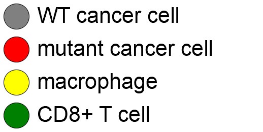
- WT cancer cells: Proliferate and release a signal that will stimulate an immune response. Cancer cells can transform into mutant cancer cells. Dead cells release debris. Damage increases apoptotic cell death.
- Mutant cancer cells: Proliferate but release less of the signal, as a model of immune evasion. Dead cells release debris. Damage increases apoptotic cell death.
- Macrophages: Chemotax towards the tumor signal and debris, and release a pro-inflammatory signal. They phagocytose dead cells.
- CD8+ T cells: Chemotax towards the pro-inflammatory signal and cause damage to tumor cells. As a model of immune evasion, CD8+ T cells can damage WT cancer cells faster than mutant cancer cells.
We will use the following diffusing factors:
- Tumor signal: Released by WT and mutant cells at different rates. We’ll fix a 1 min\(^{-1}\) decay rate and set the diffusion parameter to 10000 \(\mu m^2/\)min to give a 100 micron diffusion length scale.
- Pro-inflammatory signal: Released by macrophages. We’ll fix a 1 min\(^{-1}\) decay rate and set the diffusion parameter to 10000 \(\mu;m^2/\)min to give a 100 micron diffusion length scale.
- Debris: Released by dead cells. We’ll fix a 0.01 min\(^{-1}\) decay rate and choose a diffusion coefficient of 1 \(\mu;m^2/\)min for a 10 micron diffusion length scale.
In particular, we won’t worry about oxygen or resources in this model. We can use Neumann (no flux) boundary conditions.
Getting started with a template project and the graphical model builder
The PhysiCell Model Builder was developed by Randy Heiland and undergraduate researchers at Indiana University to help ease the creation of PhysiCell models, with a focus on generating correct XML configuration files that define the diffusing substrates and cell definitions. Here, we assume that you have cloned (or downloaded) the repository adjacent to your PhysiCell repository. (So that the path to PMB from PhysiCell’s root directory is ../PhysiCell-model-builder/).
Let’s start a new project (starting with the template project) from a command prompt or shell in the PhysiCell directory, and then open the model builder.
make template
make
python ../PhysiCell-model-builder/bin/pmb.py
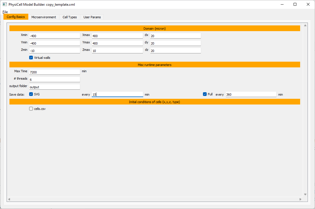
Setting up the domain
Let’s use a [-400,400] x [-400,400] 2D domain, with “virtual walls” enabled (so cells stay in the domain). We’ll run for 5760 minutes (4 days), saving SVG outputs every 15 minutes.
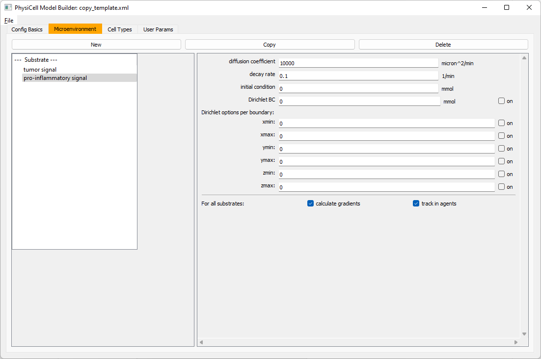
Setting up diffusing substrates
Move to the microenvironment tab. Click on substrate and rename it to tumor signal . Set the decay rate to 0.1 and diffusion parameter to 10000. Uncheck the Dirichlet condition box so that it’s a zero-flux (Neumann) boundary condition.
 Now, select
 tumor signal in the lefthand column, click copy, and rename the new substrate (substrate01) to pro-inflammatory signal with the same parameters.
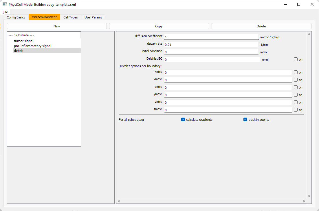
Then, copy this substrate one more time, and rename it from name debris. Set its decay rate to 0.01, and its diffusion parameter to 1.
Let’s save our work before continuing. Go to File, Save as, and save it as PhysiCell_settings.xml in your config file. (Go ahead and overwrite.)
If model builder crashes, you can reopen it, then go to File, Open, and select this file to continue editing.
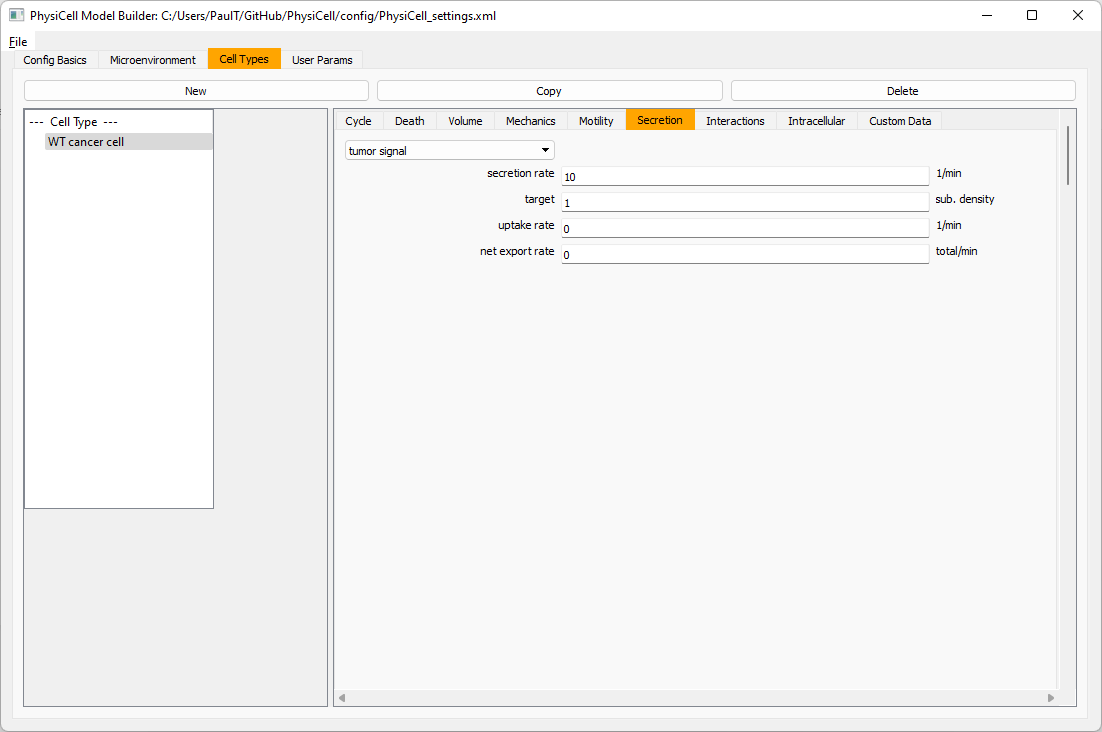
Setting up the WT cancer cells
Move to the cell types tab. Click on the default cell type on the left side, and rename it to WT cancer cell. Leave most of the parameter values at their defaults. Move to the secretion sub-tab (in phenotype). From the drop-down menu, select tumor signal. Let’s set a high secretion rate of 10.
We’ll need to set WT cells as able to mutate, but before that, the model builder needs to “know” about that cell type. So, let’s move on to the next cell type for now.
Setting up mutant tumor cells
Click the WT cancer cell in the left column, and click copy. Rename this cell type (for me, it’s cell_def03) to mutant cancer cell. Click the secretion sub-tab, and set its secretion rate of tumor signal lower to 0.1.
Set the WT mutation rate
Now that both cell types are in the simulation, we can set up mutation. Let’s suppose the mean time to a mutation is 10000 minutes, or a rate of 0.0001 min\(^{-1}\).
Click the WT cancer cell in the left column to select it. Go to the interactions tab. Go down to transformation rate, and choose mutant cancer cell from the drop-down menu. Set its rate to 0.0001.

Create macrophages
Now click on the WT cancer cell type in the left column, and click copy to create a new cell type. Click on the new type (for me cell_def04) and rename it to macrophage.
Click on cycle and change to a live cells and change from a duration representation to a transition rate representation. Keep its cycling rate at 0.
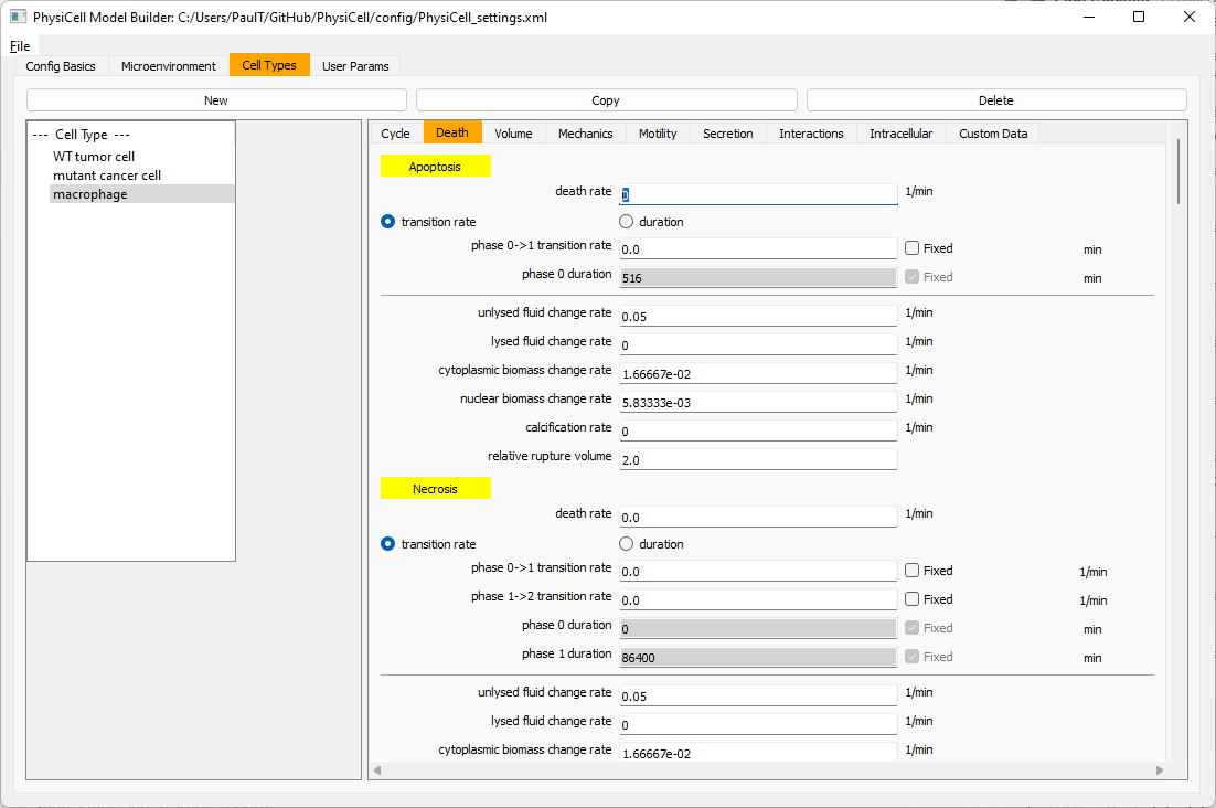
Go to death and change from duration to transition rate for both apoptosis and necrosis, and keep the death rates at 0.0
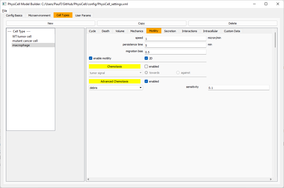
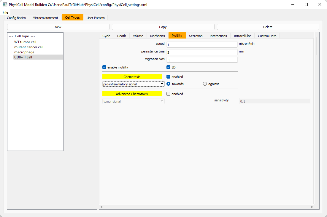
Now, go to the motility tab. Set the speed to 1 \(\mu m/\)min, persistence time to 5 min, and migration bias to 0.5. Be sure to enable motility. Then, enable advanced motility. Choose tumor signal from the drop-down and set its sensitivity to 1.0. Then choose debris from the drop-down and set its sensitivity to 0.1
Now, let’s make sure it secretes pro-inflammatory signal. Go to the secretion tab. Choose tumor signal from the drop-down, and make sure its secretion rate is 0. Then choose pro-inflammatory signal from the drop-down, set its secretion rate to 100, and its target value to 1.

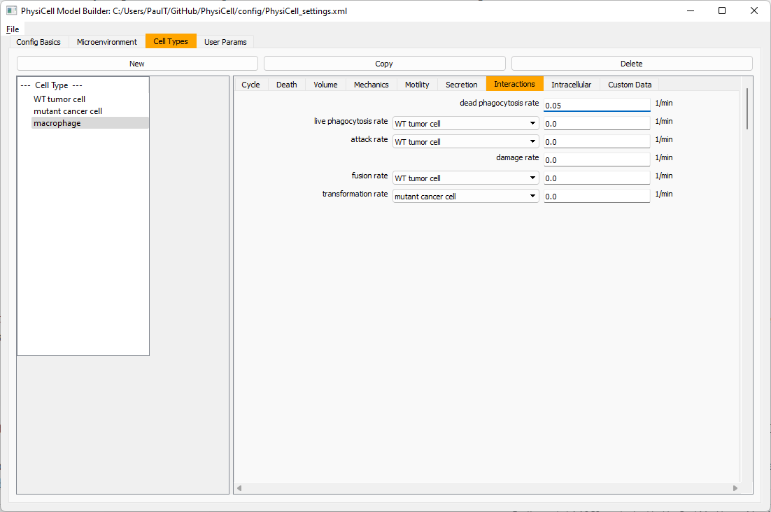
Lastly, let’s set macrophages up to phagocytose dead cells. Go to the interactions tab. Set the dead phagocytosis rate to 0.05 (so that the mean contact time to wait to eat a dead cell is 1/0.05 = 20 minutes). This would be a good time to save your work.
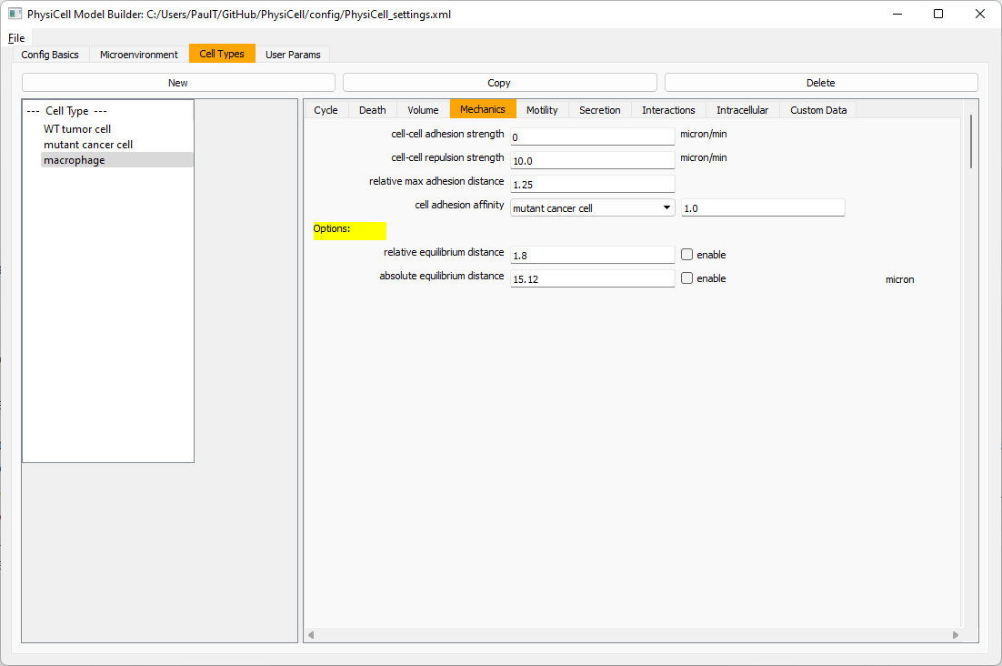
Macrophages probably shouldn’t be adhesive. So go to the mechanics sub-tab, and set the cell-cell adhesion strength to 0.0.
Create CD8+ T cells
Select macrophage on the left column, and choose copy. Rename the new cell type to CD8+ T cell. Go to the secretion sub-tab and make sure to set the secretion rate of pro-inflammatory signal to 0.0.
Now, let’s use simpler chemotaxis for these towards pro-inflammatory signal. Go to the motility tab. Uncheck advanced chemotaxis and check chemotaxis. Choose pro-inflammatory signal from the drop-down, with the towards option.
Lastly, let’s set these cells to attack WT and tumor cells. Go to the interactions tab. Set the dead phagocytosis rate to 0.
Now, let’s work on attack. Set the damage rate to 1.0. Near attack rate, choose WT tumor cell from the drop-down, and set its attack rate to 10 (so it attacks during any 0.1 minute interval). Then choose mutant tumor cell from the drop-down, and set its attack rate to 1 (as a model of immune evasion, where they are less likely to attack a non-WT tumor cell).

Set the initial cell conditions
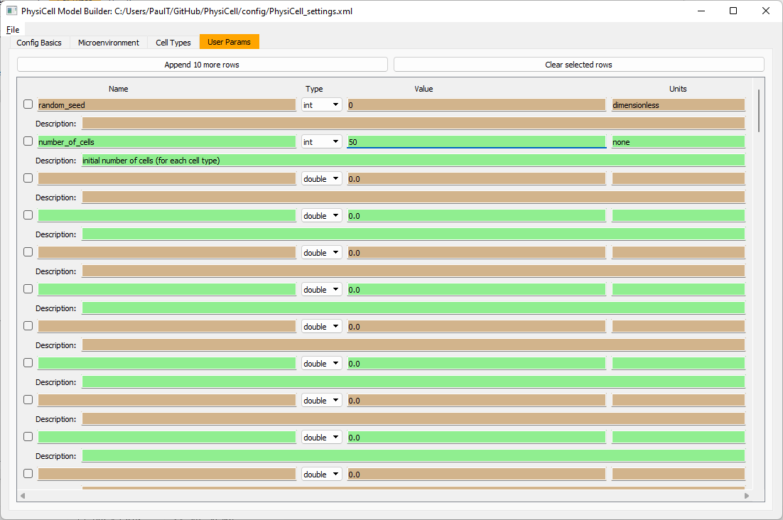
Go to the user params tab. On number of cells, choose 50. It will randomly place 50 of each cell type at the start of the simulation.
That’s all! Go to File and save (or save as), and overwrite config/PhysiCell_settings.xml. Then close the model builder.
Testing the model
Go into the PhysiCell directory. Since you already compiled, just run your model (which will use PhysiCell_settings.xml that you just saved to the config directory). For Linux or MacOS (or similar Unix-like systems):
./project
Windows users would type project without the ./ at the front.
Take a look at your SVG outputs in the output directory. You might consider making an animated gif (make gif) or a movie:
make jpeg && make movie
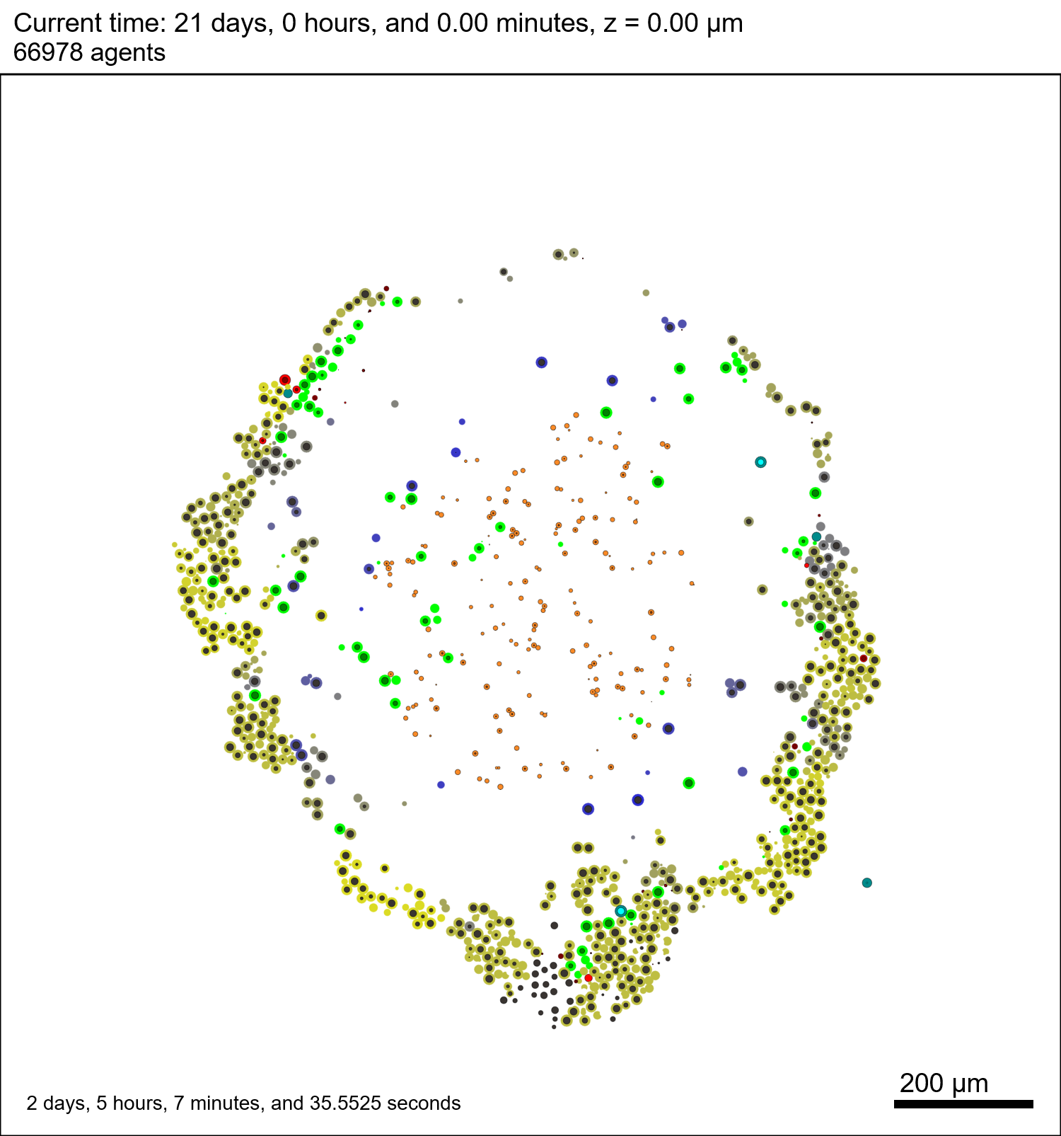
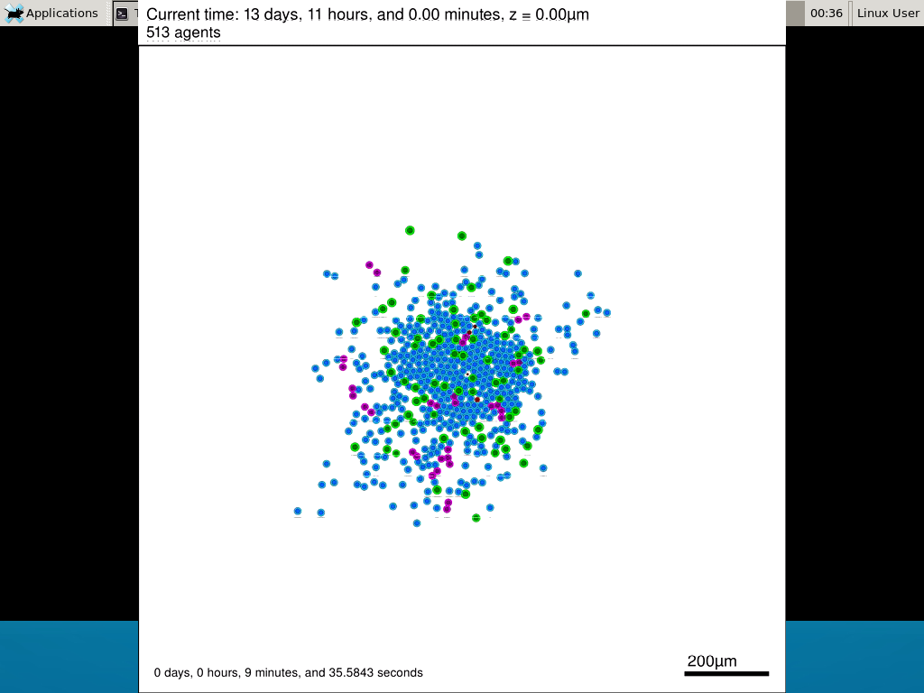
Here’s what we have.
 |
Promising! But we still need to write a little C++ so that damage kills tumor cells, and so that dead tumor cells release debris. (And we could stand to “anchor” tumor cells to ECM so they don’t get pushed around by the immune cells, but that’s a post for another day!)
Customizing the WT and mutant tumor cells with phenotype functions
First, open custom.h in the custom_modules directory, and declare a function for tumor phenotype:
void tumor_phenotype_function( Cell* pCell, Phenotype& phenotype, double dt );
Now, let’s open custom.cpp to write this function at the bottom. Here’s what we’ll do:
- If dead, set rate of debris release to 1.0 and return.
- Otherwise, we’ll set damage-based apoptosis.
- Get the base apoptosis rate
- Get the current damage
- Use a Hill response function with a half-max of 36, max apoptosis rate of 0.05 min\(^{-1}\), and a hill power of 2.0
Here’s the code:
void tumor_phenotype_function( Cell* pCell, Phenotype& phenotype, double dt )
{
   // find my cell definition
   static Cell_Definition* pCD = find_cell_definition( pCell->type_name );

   // find the index of debris in the environment
   static int nDebris = microenvironment.find_density_index( "debris" );
   static int nTS = microenvironment.find_density_index( "tumor signal" );

   // if dead: release debris. stop releasing tumor signal
   if( phenotype.death.dead == true )
   {
      phenotype.secretion.secretion_rates[nDebris] = 1;
      phenotype.secretion.saturation_densities[nDebris] = 1;

      phenotype.secretion.secretion_rates[nTS] = 0;

      // last time I'll execute this function (special optional trick)
      pCell->functions.update_phenotype = NULL;
      return;
   }

   // damage increases death

   // find death model
   static int nApoptosis =
      phenotype.death.find_death_model_index( PhysiCell_constants::apoptosis_death_model );

   double signal = pCell->state.damage; // current damage
   double base_val = pCD->phenotype.death.rates[nApoptosis]; // base death rate (from cell def)
   double max_val = 0.05; // max death rate (at large damage)

   static double damage_halfmax = 36.0;
   double hill_power = 2.0;

   // evaluate Hill response function
   double hill = Hill_response_function( signal , damage_halfmax , hill_power );
   // set "dose-dependent" death rate
   phenotype.death.rates[nApoptosis] = base_val + (max_val-base_val)*hill;

   return;
}
Now, we need to make sure we apply these functions to tumor cell. Go to `create_cell_types` and look just before we display the cell definitions. We need to:
- Search for the WT tumor cell definition
- Set the update_phenotype function for that type to the tumor_phenotype_function we just wrote
- Repeat for the mutant tumor cell type.
Here’s the code:
...
   /*
      Put any modifications to individual cell definitions here.

      This is a good place to set custom functions.
   */

   cell_defaults.functions.update_phenotype = phenotype_function;
   cell_defaults.functions.custom_cell_rule = custom_function;
   cell_defaults.functions.contact_function = contact_function;

   Cell_Definition* pCD = find_cell_definition( "WT cancer cell");
   pCD->functions.update_phenotype = tumor_phenotype_function;

   pCD = find_cell_definition( "mutant cancer cell");
   pCD->functions.update_phenotype = tumor_phenotype_function;

   /*
      This builds the map of cell definitions and summarizes the setup.
   */

   display_cell_definitions( std::cout );
   return;
}
That’s it! Let’s recompile and run!
make && ./project
And here’s the final movie.
|
Much better! Now the
Coming up next!
We will use the signal and behavior dictionaries to help us easily write C++ functions to modulate the tumor and immune cell behaviors.
Once ready, this will be posted at http://www.mathcancer.org/blog/introducing-cell-signal-and-behavior-dictionaries/.
Working with PhysiCell MultiCellDS digital snapshots in Matlab

PhysiCell 1.2.1 and later saves data as a specialized MultiCellDS digital snapshot, which includes chemical substrate fields, mesh information, and a readout of the cells and their phenotypes at single simulation time point. This tutorial will help you learn to use the matlab processing files included with PhysiCell.
This tutorial assumes you know (1) how to work at the shell / command line of your operating system, and (2) basic plotting and other functions in Matlab.
Key elements of a PhysiCell digital snapshot
A PhysiCell digital snapshot (a customized form of the MultiCellDS digital simulation snapshot) includes the following elements saved as XML and MAT files:
- output12345678.xml : This is the “base” output file, in MultiCellDS format. It includes key metadata such as when the file was created, the software, microenvironment information, and custom data saved at the simulation time. The Matlab files read this base file to find other related files (listed next). Example: output00003696.xml
- initial_mesh0.mat : This is the computational mesh information for BioFVM at time 0.0. Because BioFVM and PhysiCell do not use moving meshes, we do not save this data at any subsequent time.
- output12345678_microenvironment0.mat : This saves each biochemical substrate in the microenvironment at the computational voxels defined in the mesh (see above). Example: output00003696_microenvironment0.mat
- output12345678_cells.mat : This saves very basic cellular information related to BioFVM, including cell positions, volumes, secretion rates, uptake rates, and secretion saturation densities. Example: output00003696_cells.mat
- output12345678_cells_physicell.mat : This saves extra PhysiCell data for each cell agent, including volume information, cell cycle status, motility information, cell death information, basic mechanics, and any user-defined custom data. Example: output00003696_cells_physicell.mat
These snapshots make extensive use of Matlab Level 4 .mat files, for fast, compact, and well-supported saving of array data. Note that even if you cannot ready MultiCellDS XML files, you can work to parse the .mat files themselves.
The PhysiCell Matlab .m files
Every PhysiCell distribution includes some matlab functions to work with PhysiCell digital simulation snapshots, stored in the matlab subdirectory. The main ones are:
- composite_cutaway_plot.m : provides a quick, coarse 3-D cutaway plot of the discrete cells, with different colors for live (red), apoptotic (b), and necrotic (black) cells.
- read_MultiCellDS_xml.m : reads the “base” PhysiCell snapshot and its associated matlab files.
- set_MCDS_constants.m : creates a data structure MCDS_constants that has the same constants as PhysiCell_constants.h. This is useful for identifying cell cycle phases, etc.
- simple_cutaway_plot.m : provides a quick, coarse 3-D cutaway plot of user-specified cells.
- simple_plot.m : provides, a quick, coarse 3-D plot of the user-specified cells, without a cutaway or cross-sectional clipping plane.
A note on GNU Octave
Unfortunately, GNU octave does not include XML file parsing without some significant user tinkering. And one you’re done, it is approximately one order of magnitude slower than Matlab. Octave users can directly import the .mat files described above, but without the helpful metadata in the XML file. We’ll provide more information on the structure of these MAT files in a future blog post. Moreover, we plan to provide python and other tools for users without access to Matlab.
A sample digital snapshot
We provide a 3-D simulation snapshot from the final simulation time of the cancer-immune example in Ghaffarizadeh et al. (2017, in review) at:
The corresponding SVG cross-section for that time (through z = 0 μm) looks like this:
Unzip the sample dataset in any directory, and make sure the matlab files above are in the same directory (or in your Matlab path). If you’re inside matlab:
!unzip 3D_PhysiCell_matlab_sample.zip
Loading a PhysiCell MultiCellDS digital snapshot
Now, load the snapshot:
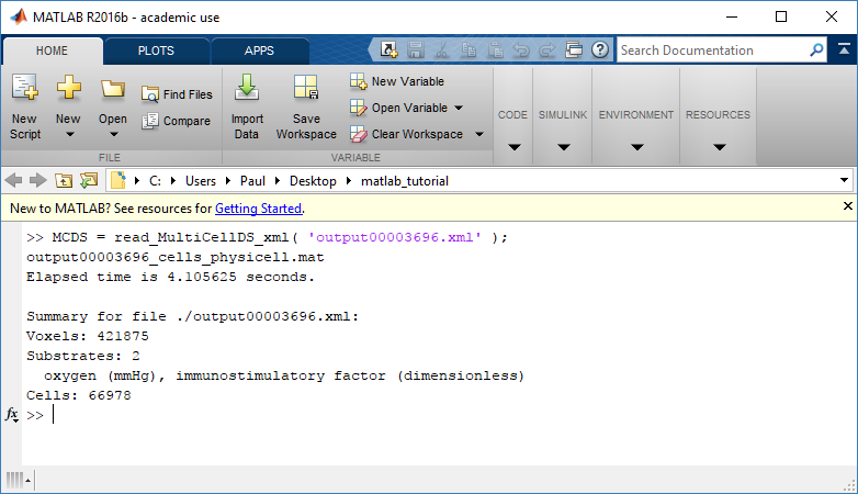
MCDS = read_MultiCellDS_xml( 'output00003696.xml');
This will load the mesh, substrates, and discrete cells into the MCDS data structure, and give a basic summary:
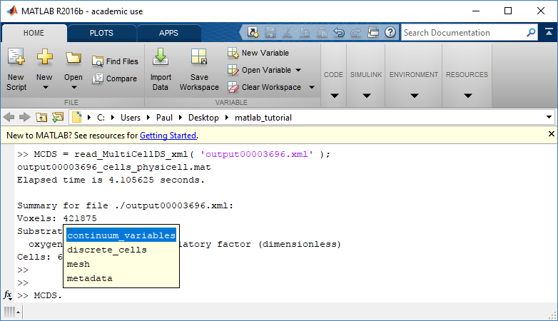
Typing ‘MCDS’ and then hitting ‘tab’ (for auto-completion) shows the overall structure of MCDS, stored as metadata, mesh, continuum variables, and discrete cells:
To get simulation metadata, such as the current simulation time, look at MCDS.metadata.current_time
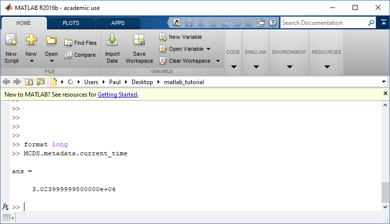
Here, we see that the current simulation time is 30240 minutes, or 21 days. MCDS.metadata.current_runtime gives the elapsed walltime to up to this point: about 53 hours (1.9e5 seconds), including file I/O time to write full simulation data once per 3 simulated minutes after the start of the adaptive immune response.
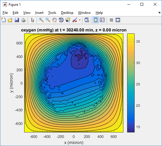
Plotting chemical substrates
Let’s make an oxygen contour plot through z = 0 μm. First, we find the index corresponding to this z-value:
k = find( MCDS.mesh.Z_coordinates == 0 );
Next, let’s figure out which variable is oxygen. Type “MCDS.continuum_variables.name”, which will show the array of variable names:
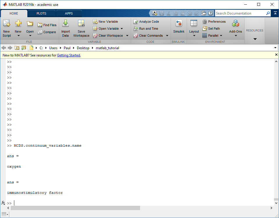
Here, oxygen is the first variable, (index 1). So, to make a filled contour plot:
contourf( MCDS.mesh.X(:,:,k), MCDS.mesh.Y(:,:,k), ...
     MCDS.continuum_variables(1).data(:,:,k) , 20 ) ;
Now, let’s set this to a correct aspect ratio (no stretching in x or y), add a colorbar, and set the axis labels, using
metadata to get labels:
axis image
colorbar
xlabel( sprintf( 'x (%s)' , MCDS.metadata.spatial_units) );
ylabel( sprintf( 'y (%s)' , MCDS.metadata.spatial_units) );
Lastly, let’s add an appropriate (time-based) title:
title( sprintf('%s (%s) at t = %3.2f %s, z = %3.2f %s', MCDS.continuum_variables(1).name , ...
     MCDS.continuum_variables(1).units , ...
     MCDS.metadata.current_time , ...
     MCDS.metadata.time_units, ...
     MCDS.mesh.Z_coordinates(k), ...
     MCDS.metadata.spatial_units ) );
Here’s the end result:
We can easily export graphics, such as to PNG format:
print( '-dpng' , 'output_o2.png' );
For more on plotting BioFVM data, see the tutorial
at http://www.mathcancer.org/blog/saving-multicellds-data-from-biofvm/
Plotting cells in space
3-D point cloud
First, let’s plot all the cells in 3D:
plot3( MCDS.discrete_cells.state.position(:,1) , MCDS.discrete_cells.state.position(:,2), ...
	MCDS.discrete_cells.state.position(:,3) , 'bo' );
At first glance, this does not look good: some cells are far out of the simulation domain, distorting the automatic range of the plot:
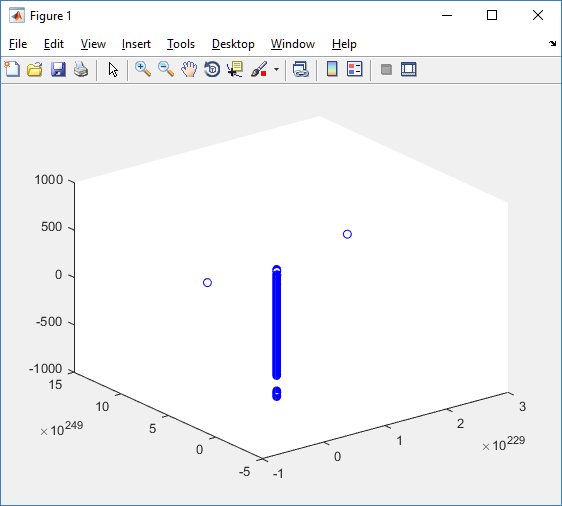
This does not ordinarily happen in PhysiCell (the default cell mechanics functions have checks to prevent such behavior), but this example includes a simple Hookean elastic adhesion model for immune cell attachment to tumor cells. In rare circumstances, an attached tumor cell or immune cell can apoptose on its own (due to its background apoptosis rate),
without “knowing” to detach itself from the surviving cell in the pair. The remaining cell attempts to calculate its elastic velocity based upon an invalid cell position (no longer in memory), creating an artificially large velocity that “flings” it out of the simulation domain. Such cells are not simulated any further, so this is effectively equivalent to an extra apoptosis event (only 3 cells are out of the simulation domain after tens of millions of cell-cell elastic adhesion calculations). Future versions of this example will include extra checks to prevent this rare behavior.
The plot can simply be fixed by changing the axis:
axis( 1000*[-1 1 -1 1 -1 1] )
axis square
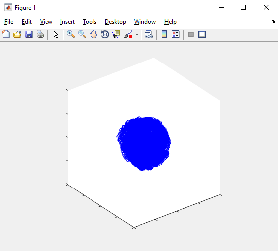
Notice that this is a very difficult plot to read, and very non-interactive (laggy) to rotation and scaling operations. We can make a slightly nicer plot by searching for different cell types and plotting them with different colors:
% make it easier to work with the cell positions;
P = MCDS.discrete_cells.state.position;

% find type 1 cells
ind1 = find( MCDS.discrete_cells.metadata.type == 1 );
% better still, eliminate those out of the simulation domain
ind1 = find( MCDS.discrete_cells.metadata.type == 1 & ...
    abs(P(:,1))' < 1000 & abs(P(:,2))' < 1000 & abs(P(:,3))' < 1000 );

% find type 0 cells
ind0 = find( MCDS.discrete_cells.metadata.type == 0 & ...
    abs(P(:,1))' < 1000 & abs(P(:,2))' < 1000 & abs(P(:,3))' < 1000 );

%now plot them
P = MCDS.discrete_cells.state.position;
plot3( P(ind0,1), P(ind0,2), P(ind0,3), 'bo' )
hold on
plot3( P(ind1,1), P(ind1,2), P(ind1,3), 'ro' )
hold off
axis( 1000*[-1 1 -1 1 -1 1] )
axis square
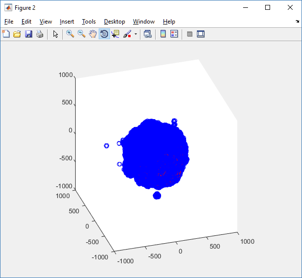
However, this isn’t much better. You can use the scatter3 function to gain more control on the size and color of the plotted cells, or even make macros to plot spheres in the cell locations (with shading and lighting), but Matlab is very slow when plotting beyond 103 cells. Instead, we recommend the faster preview functions below for data exploration, and higher-quality plotting (e.g., by POV-ray) for final publication-
Fast 3-D cell data previewers
Notice that plot3 and scatter3 are painfully slow for any nontrivial number of cells. We can use a few fast previewers to quickly get a sense of the data. First, let’s plot all the dead cells, and make them red:
clf
simple_plot( MCDS,  MCDS, MCDS.discrete_cells.dead_cells , 'r' )
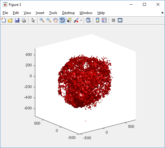
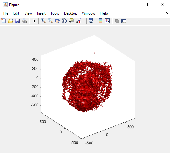
This function creates a coarse-grained 3-D indicator function (0 if no cells are present; 1 if they are), and plots a 3-D level surface. It is very responsive to rotations and other operations to explore the data. You may notice the second argument is a list of indices: only these cells are plotted. This gives you a method to select cells with specific characteristics when plotting. (More on that below.) If you want to get a sense of the interior structure, use a cutaway plot:
clf
simple_cutaway_plot( MCDS, MCDS, MCDS.discrete_cells.dead_cells , 'r' )
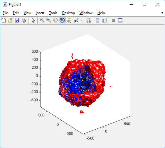
We also provide a fast “composite” cutaway which plots all live cells as red, apoptotic cells as blue (without the cutaway), and all necrotic cells as black:
clf
composite_cutaway_plot( MCDS )
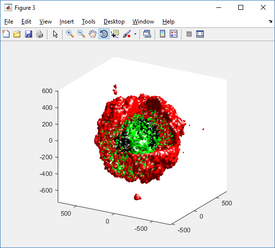
Lastly, we show an improved plot that uses different colors for the immune cells, and Matlab’s “find” function to help set up the indexing:
constants = set_MCDS_constants

% find the type 0 necrotic cells
ind0_necrotic = find( MCDS.discrete_cells.metadata.type == 0 & ...
    (MCDS.discrete_cells.phenotype.cycle.current_phase == constants.necrotic_swelling | ...
    MCDS.discrete_cells.phenotype.cycle.current_phase == constants.necrotic_lysed | ...
    MCDS.discrete_cells.phenotype.cycle.current_phase == constants.necrotic) );

% find the live type 0 cells
ind0_live = find( MCDS.discrete_cells.metadata.type == 0 & ...
    (MCDS.discrete_cells.phenotype.cycle.current_phase ~= constants.necrotic_swelling & ...
    MCDS.discrete_cells.phenotype.cycle.current_phase ~= constants.necrotic_lysed & ...
    MCDS.discrete_cells.phenotype.cycle.current_phase ~= constants.necrotic & ...
    MCDS.discrete_cells.phenotype.cycle.current_phase ~= constants.apoptotic) );

clf
% plot live tumor cells red, in cutaway view
simple_cutaway_plot( MCDS, ind0_live , 'r' );
hold on
% plot dead tumor cells black, in cutaway view
simple_cutaway_plot( MCDS, ind0_necrotic , 'k' )
% plot all immune cells, but without cutaway (to show how they infiltrate)
simple_plot( MCDS, ind1, 'g' )
hold off
A small cautionary note on future compatibility
PhysiCell 1.2.1 uses the <custom> data tag (allowed as part of the MultiCellDS specification) to encode its cell data, to allow a more compact data representation, because the current PhysiCell daft does not support such a formulation, and Matlab is painfully slow at parsing XML files larger than ~50 MB. Thus, PhysiCell snapshots are not yet fully compatible with general MultiCellDS tools, which would by default ignore custom data. In the future, we will make available converter utilities to transform “native” custom PhysiCell snapshots to MultiCellDS snapshots that encode all the cellular information in a more verbose but compatible XML format.
Closing words and future work
Because Octave is not a great option for parsing XML files (with critical MultiCellDS metadata), we plan to write similar functions to read and plot PhysiCell snapshots in Python, as an open source alternative. Moreover, our lab in the next year will focus on creating further MultiCellDS configuration, analysis, and visualization routines. We also plan to provide additional 3-D functions for plotting the discrete cells and varying color with their properties.
In the longer term, we will develop open source, stand-alone analysis and visualization tools for MultiCellDS snapshots (including PhysiCell snapshots). Please stay tuned!
Frequently Asked Questions (FAQs) for Building PhysiCell
Here, we document common problems and solutions in compiling and running PhysiCell projects.
Compiling Errors
I get the error “clang: error: unsupported option ‘-fopenmp’” when I compile a PhysiCell Project
When compiling a PhysiCell project in OSX, you may see an error like this:

This shows that clang is being used as the compiler, instead of g++. If you are using PhysiCell 1.2.2 or later, fix this error by setting the PHYSICELL_CPP environment variable. If you installed by Homebrew:
echo export PATH=/usr/local/bin:$PATH >> ~/.bash_profile
If you installed by MacPorts:
echo export PHYSICELL_CPP=g++-mp-7 >> ~/.bash_profile
To fix this error in earlier versions of PhysiCell (1.2.1 or earlier), edit your Makefile, and fix the CC line.
CC := g++-7 # use this if you installed g++ 7 by Homebrew
or
CC := g++-mp-7 # use this if you installed g++ 7 by MacPorts
If you have not installed g++ by MacPorts or Homebrew, please see the following tutorials:
When I compile, I get tons of weird “no such instruction” errors like
“no such instruction: `vmovsd (%rdx,%rax), #xmm0′” or
“no such instruction: `vfnmadd132sd (%rsi,%rax,8), $xmm5,%xmm0′”
When you compile, you may see a huge list of arcane symbols, like this:
 The “no such instruction” means that the compiler is trying to send CPU instructions (like these vmovsd lines) that your system doesn’t understand. (It’s like trying SSE4 instructions on a Pentium 4.) The first solution to try is to use a safer architecture, using the ARCH definition. Open your Makefile, and search for the ARCH line. If it isn’t set to native, then try that. If it is already set to native, try a safer, older architecture like core2 by commenting out native (add a # symbol to any Makefile line to comment it out), and uncommenting the core2 line:
# ARCH := native
ARCH := core2
“I don’t understand the ‘m’ flag!”
When you compile a project, you may see an error that looks like this:
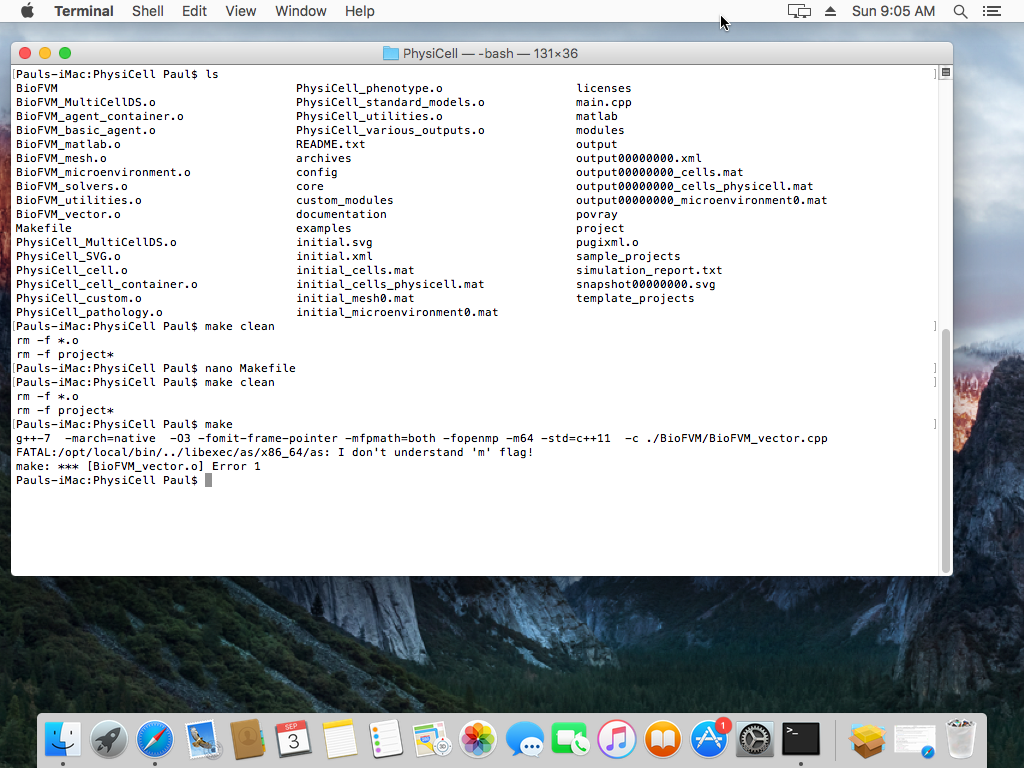
This seems to be due to incompatibilities between MacPort’s gcc chain and Homebrew (especially if you installed gcc5 in MacPorts). As we showed in this tutorial, you can open a terminal window and run a single command to fix it:
echo export PATH=/usr/bin:$PATH >> ~/.profile
Note that you’ll need to restart your terminal to fully apply the fix.
Errors Running PhysiCell
My project compiles fine, but when I run it, I get errors like “illegal instruction: 4“.
This means that PhysiCell has been compiled for the wrong architecture, and it is sending unsupported instructions to your CPU. See the “no such instruction” error above for a fix.
I fixed my Makefile, and things compiled fine, but I can’t compile a different project or the sample projects.
For PhysiCell 1.2.2 or later:
The Makefile rules for the sample projects (e.g., make biorobots-sample) overwrite the Makefile in the PhysiCell root directory, so you’ll need to return to the original state to re-populate with a new
sample project. Use
make reset
and then you’ll be good to go. As promised (below), we updated PhysiCell so that OSX users don’t need to fix the CC line for every single Makefile.
For PhysiCell 1.2.1 and earlier:
The Makefile rules for the sample projects (e.g., make biorobots-sample) overwrite the Makefile in the PhysiCell root directory, so you’ll need to re-modify the Makefile with the correct CC (and potentially ARCH) lines any time you run a template project or sample project make rule. This will be improved in future editions of PhysiCell. Sorry!!
It compiled fine, but the project crashes with “Segmentation fault: 11″, or the program just crashes with “killed.”
Everything compiles just fine and your program starts, but you may get a segmentation fault either early on, or later in your simulation. Like this:
[Screenshot soon! This error is rare.]
Or on Linux systems it might just crash with a simple “killed” message:
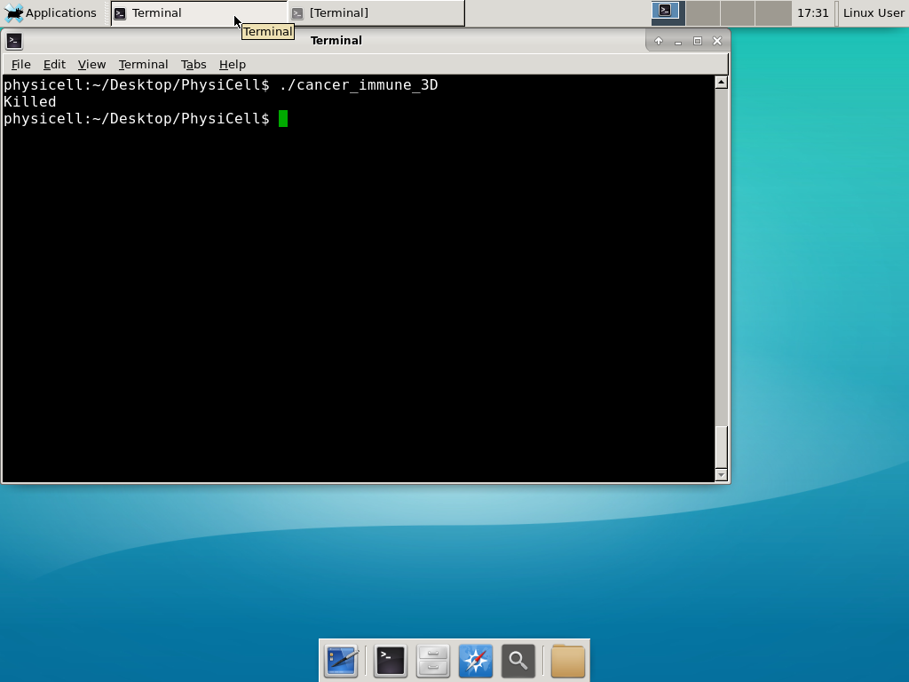
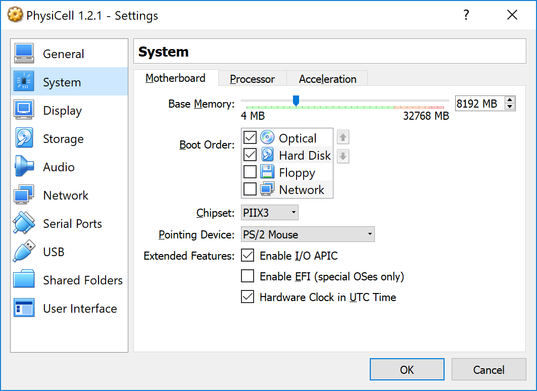
This error occurs if there is not enough (contiguous) memory to run a project. If you are running in a Virtual Machine, you can solve this by increasing the amount of memory. If you are running “natively” you may need to install more RAM or decrease the problem size (the size of the simulation domain or the number of cells). To date, we have only encountered this error on virtual machines with little memory. We recommend using 8192 MB (8 GB):
A small computational thought experiment
In Macklin (2017), I briefly touched on a simple computational thought experiment that shows that for a group of homogeneous cells, you can observe substantial heterogeneity in cell behavior. This “thought experiment” is part of a broader preview and discussion of a fantastic paper by Linus Schumacher, Ruth Baker, and Philip Maini published in Cell Systems, where they showed that a migrating collective homogeneous cells can show heterogeneous behavior when quantitated with new migration metrics. I highly encourage you to check out their work!
In this blog post, we work through my simple thought experiment in a little more detail.
Note: If you want to reference this blog post, please cite the Cell Systems preview article:
P. Macklin, When seeing isn’t believing: How math can guide our interpretation of measurements and experiments. Cell Sys., 2017 (in press). DOI: 10.1016/j.cells.2017.08.005
The thought experiment
Consider a simple (and widespread) model of a population of cycling cells: each virtual cell (with index i) has a single “oncogene” \( r_i \) that sets the rate of progression through the cycle. Between now (t) and a small time from now ( \(t+\Delta t\)), the virtual cell has a probability \(r_i \Delta t\) of dividing into two daughter cells. At the population scale, the overall population growth model that emerges from this simple single-cell model is:
\[\frac{dN}{dt} = \langle r\rangle N, \]
where \( \langle r \rangle \) the mean division rate over the cell population, and N is the number of cells. See the discussion in the supplementary information for Macklin et al. (2012).
Now, suppose (as our thought experiment) that we could track individual cells in the population and track how long it takes them to divide. (We’ll call this the division time.) What would the distribution of cell division times look like, and how would it vary with the distribution of the single-cell rates \(r_i\)?
Mathematical method
In the Matlab script below, we implement this cell cycle model as just about every discrete model does. Here’s the pseudocode:
t = 0;
while( t < t_max )
    for i=1:Cells.size()
        u = random_number();
        if( u < Cells[i].birth_rate * dt )
            Cells[i].division_time = Cells[i].age;
            Cells[i].divide();
        end
    end
    t = t+dt;
end
That is, until we’ve reached the final simulation time, loop through all the cells and decide if they should divide: For each cell, choose a random number between 0 and 1, and if it’s smaller than the cell’s division probability (\(r_i \Delta t\)), then divide the cell and write down the division time.
As an important note, we have to track the same cells until they all divide, rather than merely record which cells have divided up to the end of the simulation. Otherwise, we end up with an observational bias that throws off our recording. See more below.
The sample code
You can download the Matlab code for this example at:
http://MathCancer.org/files/matlab/thought_experiment_matlab(Macklin_Cell_Systems_2017).zip
Extract all the files, and run “thought_experiment” in Matlab (or Octave, if you don’t have a Matlab license or prefer an open source platform) for the main result.
All these Matlab files are available as open source, under the GPL license (version 3 or later).
Results and discussion
First, let’s see what happens if all the cells are identical, with \(r = 0.05 \textrm{ hr}^{-1}\). We run the script, and track the time for each of 10,000 cells to divide. As expected by theory (Macklin et al., 2012) (but perhaps still a surprise if you haven’t looked), we get an exponential distribution of division times, with mean time \(1/\langle r \rangle\):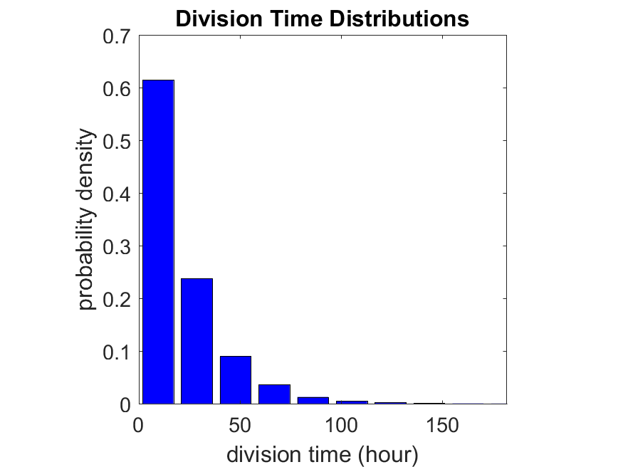
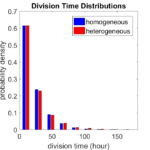
So even in this simple model, a homogeneous population of cells can show heterogeneity in their behavior. Here’s the interesting thing: let’s now give each cell its own division parameter \(r_i\) from a normal distribution with mean \(0.05 \textrm{ hr}^{-1}\) and a relative standard deviation of 25%: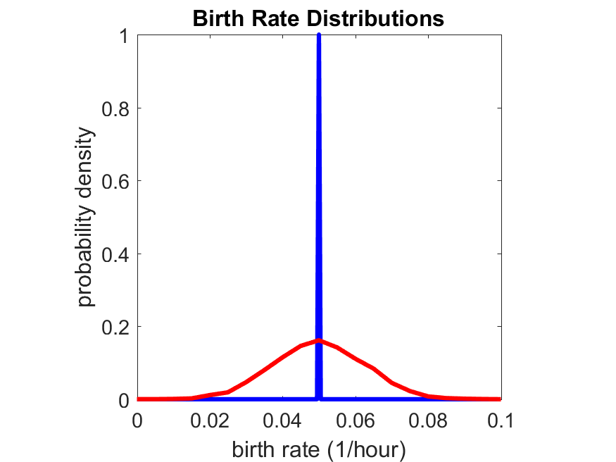
If we repeat the experiment, we get the same distribution of cell division times!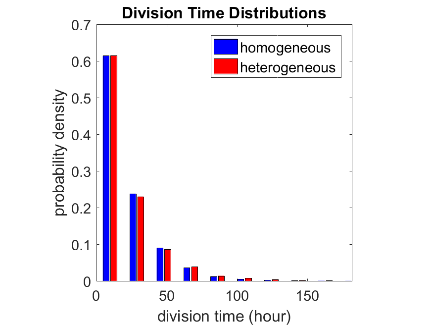
So in this case, based solely on observations of the phenotypic heterogeneity (the division times), it is impossible to distinguish a “genetically” homogeneous cell population (one with identical parameters) from a truly heterogeneous population. We would require other metrics, like tracking changes in the mean division time as cells with a higher \(r_i\) out-compete the cells with lower \(r_i\).
Lastly, I want to point out that caution is required when designing these metrics and single-cell tracking. If instead we had tracked all cells throughout the simulated experiment, including new daughter cells, and then recorded the first 10,000 cell division events, we would get a very different distribution of cell division times: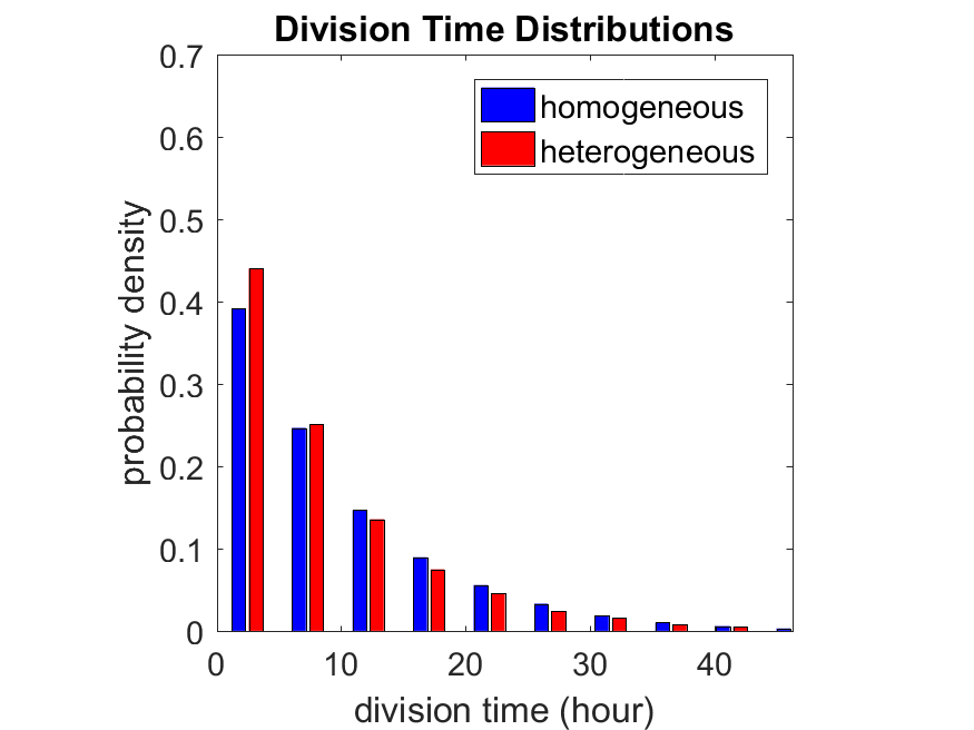
By only recording the division times for the cells that have divided, and not those that haven’t, we bias our observations towards cells with shorter division times. Indeed, the mean division time for this simulated experiment is far lower than we would expect by theory. You can try this one by running “bad_thought_experiment”.
Further reading
This post is an expansion of our recent preview in Cell Systems in Macklin (2017):
P. Macklin, When seeing isn’t believing: How math can guide our interpretation of measurements and experiments. Cell Sys., 2017 (in press). DOI: 10.1016/j.cells.2017.08.005
And the original work on apparent heterogeneity in collective cell migration is by Schumacher et al. (2017):
L. Schumacher et al., Semblance of Heterogeneity in Collective Cell Migration. Cell Sys., 2017 (in press). DOI: 10.1016/j.cels.2017.06.006
You can read some more on relating exponential distributions and Poisson processes to common discrete mathematical models of cell populations in Macklin et al. (2012):
P. Macklin, et al., Patient-calibrated agent-based modelling of ductal carcinoma in situ (DCIS): From microscopic measurements to macroscopic predictions of clinical progression. J. Theor. Biol. 301:122-40, 2012. DOI: 10.1016/j.jtbi.2012.02.002.
Lastly, I’d be delighted if you took a look at the open source software we have been developing for 3-D simulations of multicellular systems biology:
http://OpenSource.MathCancer.org
And you can always keep up-to-date by following us on Twitter: @MathCancer.
Getting started with a PhysiCell Virtual Appliance
Note: This is part of a series of “how-to” blog posts to help new users and developers of BioFVM and PhysiCell. This guide is for for users in OSX, Linux, or Windows using the VirtualBox virtualization software to run a PhysiCell virtual appliance.
These instructions should get you up and running without needed to install a compiler, makefile capabilities, or any other software (beyond the virtual machine and the PhysiCell virtual appliance). We note that using the PhysiCell source with your own compiler is still the preferred / ideal way to get started, but the virtual appliance option is a fast way to start even if you’re having troubles setting up your development environment.
What’s a Virtual Machine? What’s a Virtual Appliance?
A virtual machine is a full simulated computer (with its own disk space, operating system, etc.) running on another. They are designed to let a user test on a completely different environment, without affecting the host (main) environment. They also allow a very robust way of taking and reproducing the state of a full working environment.
A virtual appliance is just this: a full image of an installed system (and often its saved state) on a virtual machine, which can easily be installed on a new virtual machine. In this tutorial, you will download our PhysiCell virtual appliance and use its pre-configured compiler and other tools.
What you’ll need:
- VirtualBox: This is a free, cross-platform program to run virtual machines on OSX, Linux, Windows, and other platforms. It is a safe and easy way to install one full operating (a client system) on your main operating system (the host system). For us, this means that we can distribute a fully working Linux environment with a working copy of all the tools you need to compile and run PhysiCell. As of August 1, 2017, this will download Version 5.1.26.
- Download here: https://www.virtualbox.org/wiki/Downloads
- PhysiCell Virtual Appliance: This is a single-file distribution of a virtual machine running Alpine Linux, including all key tools needed to compile and run PhysiCell. As of July 31, 2017, this will download PhysiCell 1.2.2 with g++ 6.3.0.
- Download here: https://sourceforge.net/projects/physicell/files/PhysiCell/
- (Browse to a version of PhysiCell, and download the file that ends in “.ova”.)
- Version 1.2.0: http://bit.ly/2vY51P1 [sf.net]
- Download here: https://sourceforge.net/projects/physicell/files/PhysiCell/
- A computer with hardware support for virtualization: Your CPU needs to have hardware support for virtualization (almost all of them do now), and it has to be enabled in your BIOS. Consult your computer maker on how to turn this on if you get error messages later.
Main steps:
1) Install VirtualBox.
Double-click / open the VirtualBox download. Go ahead and accept all the default choices. If asked, go ahead and download/install the extensions pack.
2) Import the PhysiCell Virtual Appliance
Go the “File” menu and choose “Import Virtual Appliance”. Browse to find the .ova file you just downloaded.
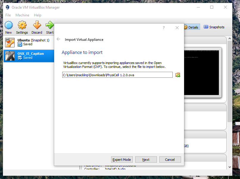
Click on “Next,” and import with all the default options. That’s it!
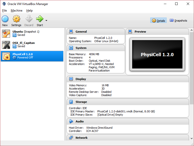
3) [Optional] Change settings
You most likely won’t need this step, but you can increase/decrease the amount of RAM used for the virtual machine if you select the PhysiCell VM, click the Settings button (orange gear), and choose “System”: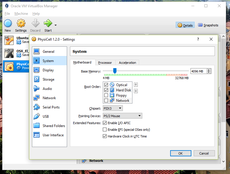 We set the Virtual Machine to have 4 GB of RAM. If you have a machine with lots of RAM (16 GB or more), you may want to set this to 8 GB.
Also, you can choose how many virtual CPUs to give to your VM: 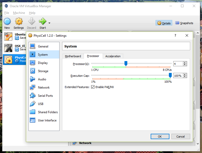
We selected 4 when we set up the Virtual Appliance, but you should match the number of physical processor cores on your machine. In my case, I have a quad core processor with hyperthreading. This means 4 real cores, 8 virtual cores, so I select 4 here.
4) Start the Virtual Machine and log in
Select the PhysiCell machine, and click the green “start” button. After the virtual machine boots (with the good old LILO boot manager that I’ve missed), you should see this:
Click the "More ..." button, and log in with username: physicell, password: physicell
5) Test the compiler and run your first simulation
Notice that PhysiCell is already there on the desktop in the PhysiCell folder. Right-click, and choose “open terminal here.” You’ll already be in the main PhysiCell root directory. 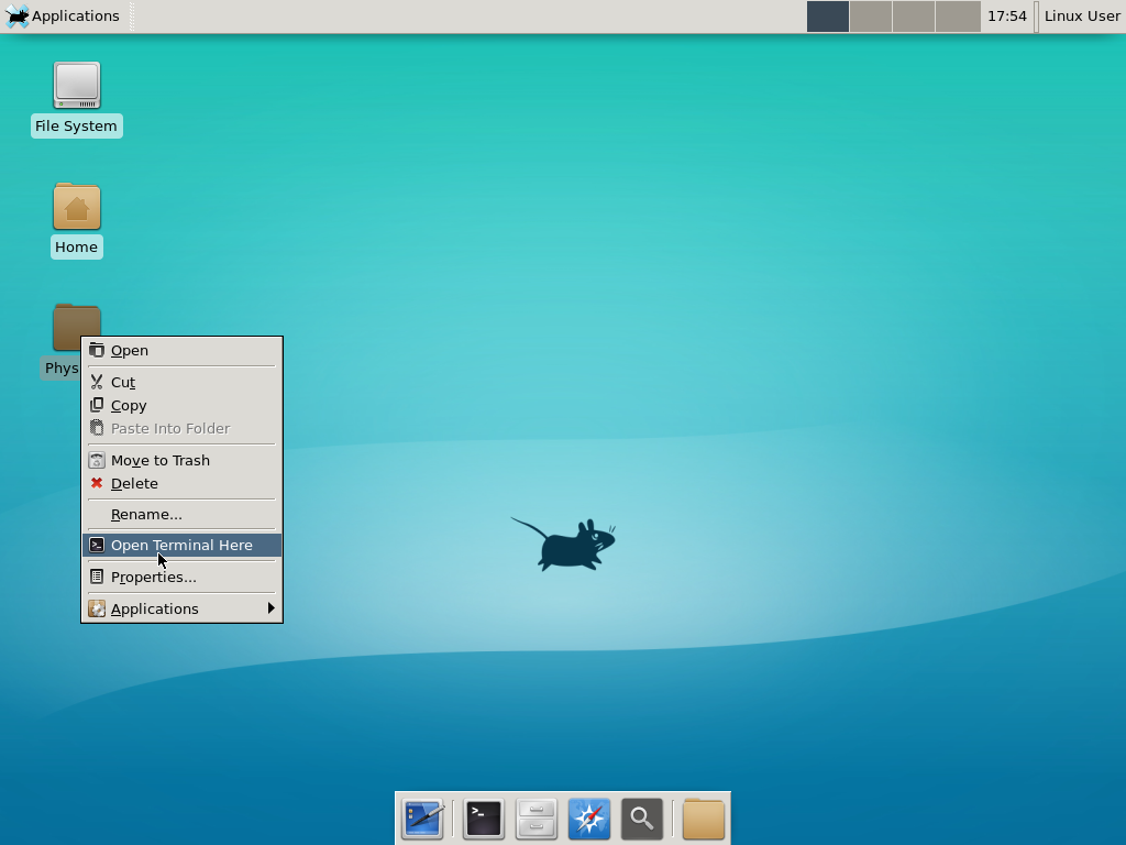
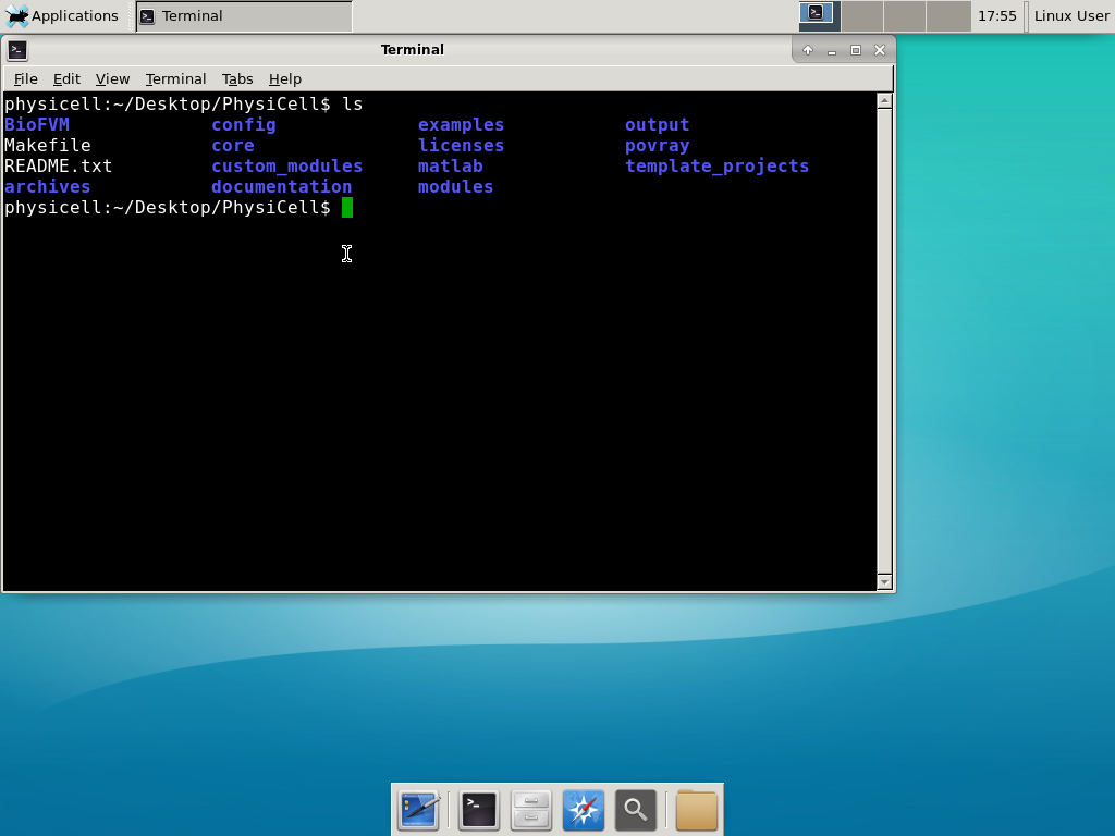
Now, let’s compile your first project! Type “make template2D && make” 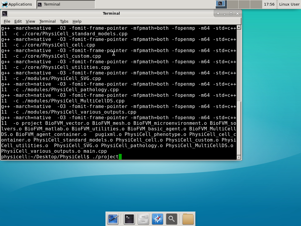 And run your project! Type “./project” and let it go!
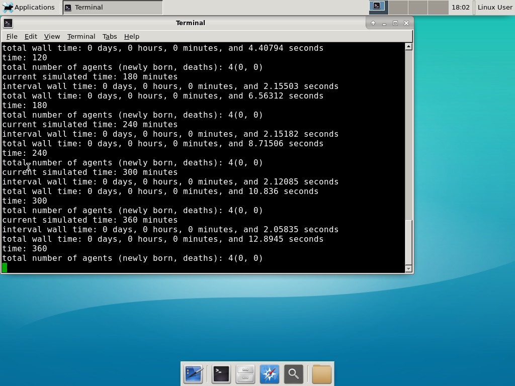 Go ahead and run either the first few days of the simulation (until about 7200 minutes), then hit <control>-C to cancel out. Or run the whole simulation–that’s fine, too.
6) Look at the results
We bundled a few tools to easily look at results. First, ristretto is a very fast image viewer. Let’s view the SVG files: 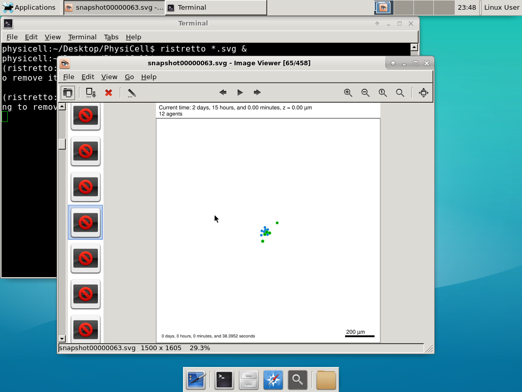 As a nice tip, you can press the left and right arrows to advance through the SVG images, or hold the right arrow down to advance through quickly.
Now, let’s use ImageMagick to convert the SVG files into JPG file: call “magick mogrify -format jpg snap*.svg”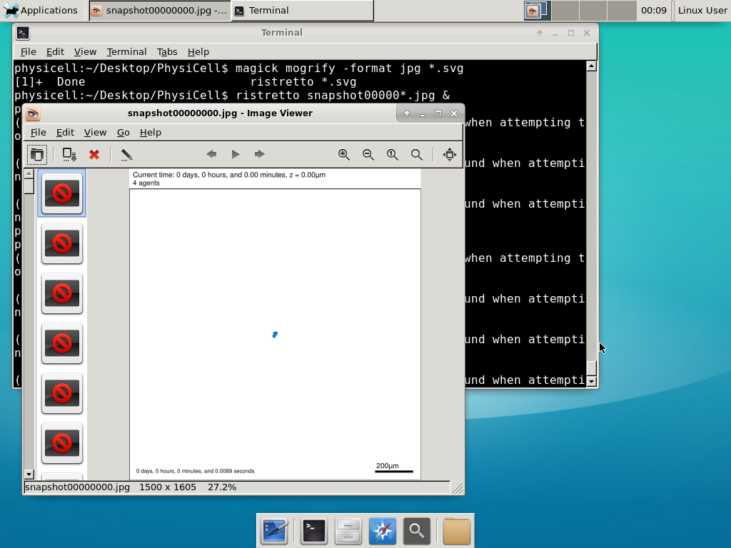
Next, let’s turn those images into a movie. I generally create moves that are 24 frames pers se, so that 1 second of the movie is 1 hour of simulations time. We’ll use mencoder, with options below given to help get a good quality vs. size tradeoff: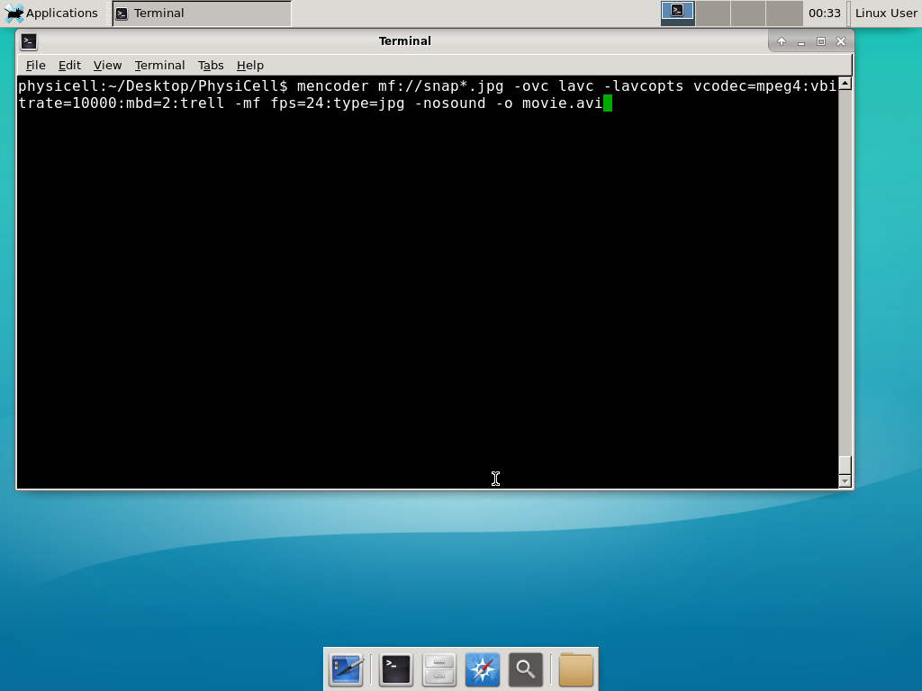
When you’re done, view the movie with mplayer. The options below scale the window to fit within the virtual monitor:
If you want to loop the movie, add “-loop 999” to your command.
7) Get familiar with other tools
Use nano (useage: nano <filename>) to quickly change files at the command line. Hit <control>-O to save your results. Hit <control>-X to exit. <control>-W will search within the file.
Use nedit (useage: nedit <filename> &) to open up one more text files in a graphical editor. This is a good way to edit multiple files at once.
Sometimes, you need to run commands at elevated (admin or root) privileges. Use sudo. Here’s an example, searching the Alpine Linux package manager apk for clang:
physicell:~$ sudo apk search gcc
[sudo] password for physicell:
physicell:~$ sudo apk search clang
clang-analyzer-4.0.0-r0
clang-libs-4.0.0-r0
clang-dev-4.0.0-r0
clang-static-4.0.0-r0
emscripten-fastcomp-1.37.10-r0
clang-doc-4.0.0-r0
clang-4.0.0-r0
physicell:~/Desktop/PhysiCell$
If you want to install clang/llvm (as an alternative compiler):
physicell:~$ sudo apk add gcc
[sudo] password for physicell:
physicell:~$ sudo apk search clang
clang-analyzer-4.0.0-r0
clang-libs-4.0.0-r0
clang-dev-4.0.0-r0
clang-static-4.0.0-r0
emscripten-fastcomp-1.37.10-r0
clang-doc-4.0.0-r0
clang-4.0.0-r0
physicell:~/Desktop/PhysiCell$
Notice that it asks for a password: use the password for root (which is physicell).
8) [Optional] Configure a shared folder
Coming soon.
Why both with zipped source, then?
Given that we can get a whole development environment by just downloading and importing a virtual appliance, why
bother with all the setup of a native development environment, like this tutorial (Windows) or this tutorial (Mac)?
One word: performance. In my testing, I still have not found the performance running inside a
virtual machine to match compiling and running directly on your system. So, the Virtual Appliance is a great
option to get up and running quickly while trying things out, but I still recommend setting up natively with
one of the tutorials I linked in the preceding paragraphs.
What’s next?
In the coming weeks, we’ll post further tutorials on using PhysiCell. In the meantime, have a look at the
PhysiCell project website, and these links as well:
- BioFVM on MathCancer.org: http://BioFVM.MathCancer.org
- BioFVM on SourceForge: http://BioFVM.sf.net
- BioFVM Method Paper in BioInformatics: http://dx.doi.org/10.1093/bioinformatics/btv730
- PhysiCell on MathCancer.org: http://PhysiCell.MathCancer.org
- PhysiCell on Sourceforge: http://PhysiCell.sf.net
- PhysiCell Method Paper (preprint): https://doi.org/10.1101/088773
- PhysiCell tutorials: [click here]
Moving the blog to MathCancer.org
Hi, everyone!
Blogspot has been a great platform for me, but in the end, editing posts with source code and mathematics has been too much of a headache in the neglected blogspot and google UIs.
Elsewhere in the universe, WordPress has developed and encouraged a great ecosystem of plugins that let you do LaTeX and code syntax highlighting directly in your posts with ease. I can’t spend hours and hours on fixing mangled posts. It’s time to move on.
So as of today, I am moving to a self-hosted blog at http://MathCancer.org/blog/
I will leave old posts at http://MathCancer.blogspot.com and gradually migrate them here to MathCancer.org/blog. Thanks for following me over the last few years.
Return to News • Return to MathCancer • Follow @MathCancer
Banner and Logo Contest : MultiCellDS Project
As the MultiCellDS (multicellular data standards) project continues to ramp up, we could use some artistic skill.
Right now, we don’t have a banner (aside from a fairly barebones placeholder using a lovely LCARS font) or a logo. While I could whip up a fancier banner and logo, I have a feeling that there is much better talent out there. So, let’s have a contest!
Here are the guidelines and suggestions:
- The banner should use the text MultiCellDS Project. It’s up to artist (and the use) whether the “multicellular data standards” part gets written out more fully (e.g., below the main part of the banner).
- The logo should be shorter and easy to use on other websites. I’d suggest MCDS, stylized similarly to the main banner.
- Think of MultiCell as a prefix: MultiCellDS, MultiCellXML, MultiCellHDF, MultiCellDB. So, the “banner” version should be extensible to new directions on the project.
- The banner and logo should be submitted in a vector graphics format, with all source.
- It goes without saying that you can’t use clip art that you don’t have rights to. (i.e., use your own artwork or photos, or properly-attributed creative commons-licensed art.)
- The banner and logo need to belong to the MultiCellDS project once done.
- We may do some final tweaks and finalization on the winning design for space or other constraints. But this will be done in full consultation with the winner.
So, what are the perks for winning?
- Permanent link to your personal research / profession page crediting you as the winner.
- A blog/post detailing how awesome you and your banner and logo are.
- Beer / coffee is on me next time I see you. SMB 2015 in Atlanta might be a good time to do it!
- If we ever make t-shirts, I’ll buy yours for you. :-)
- You get to feel good for being awesome and helping out the project!
So, please post here, on the @MultiCellDS twitter feed, or contact me if you’re interested. Once I get a sense of interest, I’ll set a deadline for submissions and “voting” procedures.
Thanks!!
2015 Speaking Schedule
Here is my current speaking schedule for 2015. Please join me if you can!
- Feb. 13, 2015: Seminar at the Institute for Scientific Computing Research, Lawrence Livermore National Laboratory (LLNL)
- Title: Scalable 3-D Agent-Based Simulations of Cells and Tissues in Biology and Cancer [abstract]
See Also:
2014 Speaking Schedule
Here is my current speaking schedule for 2014. Please join me if you can!
- Feb. 16, 2014: American Association for the Advancement of Science (AAAS) Annual Meeting, Chicago
- Title: Integrating Next-Generation Computational Models of Cancer Progression and Outcome [abstract]
- invited by the National Cancer Institute
- May 9, 2014: European Society for Medical Oncology (ESMO) 2014 IMPAKT Breast Cancer Conference, Brussels, Belgium
- Title: Calibrating breast cancer simulations with patient pathology: Progress and future steps [programme]
- Plenary talk
- May 13, 2014: Wolfson Centre for Mathematical Biology at the University of Oxford, Oxford, UK
- Title: Advances in parallelized 3-D agent-based cancer modeling and digital cell lines [abstract]
- June 19, 2014: Biostatistics Seminar, University of Southern California, Los Angeles
- Title: Simulating 3-D systems of 500k cells with an agent-based model, and digital cell lines [link]
- Aug. 18, 2014: COMBINE (Computational Modeling in Biology Network) 2014 Symposium, University of Southern California, Los Angeles
- Title: Digital cell lines and MultiCellDS: Standardizing cell phenotype data for data-driven cancer simulations[Program]
See Also:
Website updates …
I’m in the process of rolling out some updates to my website. The first thing you’ll see is a new talk / tutorial on computational modeling of biological processes, based upon my recent talk at the USC PS-OC Short Course in October 2013. I’ll make another post here when it’s ready. It will include MATLAB source code to run through the models.
In the medium term, I hope to update my list of projects to better reflect current efforts by my lab, particularly in (1) integrative modeling of cancer metastases using high-throughput in vitro experiments and sophisticated bioengineered tissues for calibration and validation, and (2) development of standardizations for cell- and tissue-scale models and experiments.
In the longer term, I hope to switch my website layout a bit to be more like the USC PSOC website. I wrote that site about a year ago, and I like the CSS and structure a lot better. :-)