Tag: tutorial
Introducing cell interactions & transformations
Introduction
PhysiCell 1.10.0 introduces a number of new features designed to simplify modeling of complex interactions and transformations. This blog post will introduce the underlying mathematics and show a complete example. We will teach this and other examples in greater depth at our upcoming Virtual PhysiCell Workshop & Hackathon (July 24-30, 2022). (Apply here!!)
Cell Interactions
In the past, it has been possible to model complex cell-cell interactions (such as those needed for microecology and immunology) by connecting basic cell functions for interaction testing and custom functions. In particular, these functions were used for the COVID19 Coalition’s open source model of SARS-CoV-2 infections and immune responses. We now build upon that work to standardize and simplify these processes, making use of the cell’s state.neighbors (a list of all cells deemed to be within mechanical interaction distance).
All the parameters for cell-cell interactions are stored in cell.phenotype.cell_interactions.
Phagocytosis
A cell can phagocytose (ingest) another cell, with rates that vary with the cell’s live/dead status or the cell type. In particular, we store:
- double dead_phagocytosis_rate : This is the rate at which a cell can phagocytose a dead cell of any type.
std::vector<double> live_phagocytosis_rates: This is a vector of phagocytosis rates for live cells of specific types. If there are n cell definitions in the simulation, then there are n rates in this vector. Please note that the index i for any cell type is its index in the list of cell definitions, not necessarily the ID of its cell definition. For safety, use one of the following to determine that index:find_cell_definition_index( int type_ID ): search for the cell definition’s index by its type ID (cell.type)find_cell_definition_index( std::string type_name ): search for the cell definition’s index by its human-readable type name (cell.type_name)
We also supply a function to help access these live phagocytosis rates.
- double& live_phagocytosis_rate( std::string type_name ) : Directly access the cell’s rate of phagocytosing the live cell type by its human-readable name. For example,
pCell->phenotype.cell_interactions.live_phagocytosis_rate( "tumor cell" ) = 0.01;
At each mechanics time step (with duration \(\Delta t\), default 0.1 minutes), each cell runs through its list of neighbors. If the neighbor is dead, its probability of phagocytosing it between \(t\) and \(t+\Delta t\) is
\[ \verb+dead_phagocytosis_rate+ \cdot \Delta t\]
If the neighbor cell is alive and its type has index j, then its probability of phagocytosing the cell between \(t\) and \(t+\Delta t\) is
\[ \verb+live_phagocytosis_rates[j]+ \cdot \Delta t\]
PhysiCell’s standardized phagocytosis model does the following:
- The phagocytosing cell will absorb the phagocytosed cell’s total solid volume into the cytoplasmic solid volume
- The phagocytosing cell will absorb the phagocytosed cell’s total fluid volume into the fluid volume
- The phagocytosing cell will absorb all of the phagocytosed cell’s internalized substrates.
- The phagocytosed cell is set to zero volume, flagged for removal, and set to not mechanically interact with remaining cells.
- The phagocytosing cell does not change its target volume. The standard volume model will gradually “digest” the absorbed volume as the cell shrinks towards its target volume.
Cell Attack
A cell can attack (cause damage to) another live cell, with rates that vary with the cell’s type. In particular, we store:
- double damage_rate : This is the rate at which a cell causes (dimensionless) damage to a target cell. The cell’s total damage is stored in cell.state.damage. The total integrated attack time is stored in
cell.state.total_attack_time. std::vector<double> attack_rates: This is a vector of attack rates for live cells of specific types. If there are n cell definitions in the simulation, then there are n rates in this vector. Please note that the index i for any cell type is its index in the list of cell definitions, not necessarily the ID of its cell definition. For safety, use one of the following to determine that index:find_cell_definition_index( int type_ID ): search for the cell definition’s index by its type ID (cell.type)find_cell_definition_index( std::string type_name ): search for the cell definition’s index by its human-readable type name (cell.type_name)
We also supply a function to help access these attack rates.
- double& attack_rate( std::string type_name ) : Directly access the cell’s rate of attacking the live cell type by its human-readable name. For example,
pCell->phenotype.cell_interactions.attack_rate( "tumor cell" ) = 0.01;
At each mechanics time step (with duration \(\Delta t\), default 0.1 minutes), each cell runs through its list of neighbors. If the neighbor cell is alive and its type has index j, then its probability of attacking the cell between \(t\) and \(t+\Delta t\) is
\[ \verb+attack_rates[j]+ \cdot \Delta t\]
To attack the cell:
- The attacking cell will increase the target cell’s damage by \( \verb+damage_rate+ \cdot \Delta t\).
- The attacking cell will increase the target cell’s total attack time by \(\Delta t\).
Note that this allows us to have variable rates of damage (e.g., some immune cells may be “worn out”), and it allows us to distinguish between damage and integrated interaction time. (For example, you may want to write a model where damage can be repaired over time.)
As of this time, PhysiCell does not have a standardized model of death in response to damage. It is up to the modeler to vary a death rate with the total attack time or integrated damage, based on their hypotheses. For example:
\[ r_\textrm{apoptosis} = r_\textrm{apoptosis,0} + \left( r_\textrm{apoptosis,max} – r_\textrm{apoptosis,0} \right) \cdot \frac{ d^h }{ d_\textrm{halfmax}^h + d^h } \]
In a phenotype function, we might write this as:
void damage_response( Cell* pCell, Phenotype& phenotype, double dt )
{ // get the base apoptosis rate from our cell definition
     Cell_Definition* pCD = find_cell_definition( pCell->type_name );
     double apoptosis_0 = pCD->phenotype.death.rates[0];
     double apoptosis_max = 100 * apoptosis_0;
     double half_max = 2.0;
     double damage = pCell->state.damage;
     phenotype.death.rates[0] = apoptosis_0 +
(apoptosis_max -apoptosis_0) * Hill_response_function(d,half_max,1.0);
     return;
}
Cell Fusion
A cell can fuse with another live cell, with rates that vary with the cell’s type. In particular, we store:
std::vector<double> fusion_rates: This is a vector of fusion rates for live cells of specific types. If there are n cell definitions in the simulation, then there are n rates in this vector. Please note that the index i for any cell type is its index in the list of cell definitions, not necessarily the ID of its cell definition. For safety, use one of the following to determine that index:find_cell_definition_index( int type_ID ): search for the cell definition’s index by its type ID (cell.type)find_cell_definition_index( std::string type_name ): search for the cell definition’s index by its human-readable type name (cell.type_name)
We also supply a function to help access these fusion rates.
- double& fusion_rate( std::string type_name ) : Directly access the cell’s rate of fusing with the live cell type by its human-readable name. For example,
pCell->phenotype.cell_interactions.fusion_rate( "tumor cell" ) = 0.01;
At each mechanics time step (with duration \(\Delta t\), default 0.1 minutes), each cell runs through its list of neighbors. If the neighbor cell is alive and its type has index j, then its probability of fusing with the cell between \(t\) and \(t+\Delta t\) is
\[ \verb+fusion_rates[j]+ \cdot \Delta t\]
PhysiCell’s standardized fusion model does the following:
- The fusing cell will absorb the fused cell’s total cytoplasmic solid volume into the cytoplasmic solid volume
- The fusing cell will absorb the fused cell’s total nuclear volume into the nuclear solid volume
- The fusing cell will keep track of its number of nuclei in
state.number_of_nuclei. (So, if the fusing cell has 3 nuclei and the fused cell has 2 nuclei, then the new cell will have 5 nuclei.) - The fusing cell will absorb the fused cell’s total fluid volume into the fluid volume
- The fusing cell will absorb all of the fused cell’s internalized substrates.
- The fused cell is set to zero volume, flagged for removal, and set to not mechanically interact with remaining cells.
- The fused cell will be moved to the (volume weighted) center of mass of the two original cells.
- The fused cell does change its target volume to the sum of the original two cells’ target volumes. The combined cell will grow / shrink towards its new target volume.
Cell Transformations
A live cell can transform to another type (e.g., via differentiation). We store parameters for cell transformations in cell.phenotype.cell_transformations, particularly:
std::vector<double> transformation_rates: This is a vector of transformation rates from a cell’s current to type to one of the other cell types. If there are n cell definitions in the simulation, then there are n rates in this vector. Please note that the index i for any cell type is its index in the list of cell definitions, not necessarily the ID of its cell definition. For safety, use one of the following to determine that index:find_cell_definition_index( int type_ID ): search for the cell definition’s index by its type ID (cell.type)find_cell_definition_index( std::string type_name ): search for the cell definition’s index by its human-readable type name (cell.type_name)
We also supply a function to help access these transformation rates.
- double& transformation_rate( std::string type_name ) : Directly access the cell’s rate of transforming into a specific cell type by searching for its human-readable name. For example,
pCell->phenotype.cell_transformations.transformation_rate( "mutant tumor cell" ) = 0.01;
At each phenotype time step (with duration \(\Delta t\), default 6 minutes), each cell runs through the vector of transformation rates. If a (different) cell type has index j, then the cell’s probability transforming to that type between \(t\) and \(t+\Delta t\) is
\[ \verb+transformation_rates[j]+ \cdot \Delta t\]
PhysiCell uses the built-in Cell::convert_to_cell_definition( Cell_Definition& ) for the transformation.
Other New Features
This release also includes a number of handy new features:
Advanced Chemotaxis
After setting chemotaxis sensitivities in phenotype.motility and enabling the feature, cells can chemotax based on linear combinations of substrate gradients.
std::vector<double> phenotype.motility.chemotactic_sensitivitiesis a vector of chemotactic sensitivities, one for each substrate in the environment. By default, these are all zero for backwards compatibility. A positive sensitivity denotes chemotaxis up a corresponding substrate’s gradient (towards higher values), whereas a negative sensitivity gives chemotaxis against a gradient (towards lower values).- For convenience, you can access (read and write) a substrate’s chemotactic sensitivity via
phenotype.motility.chemotactic_sensitivity(name)wherenameis the human-readable name of a substrate in the simulation. - If the user sets
cell.cell_functions.update_migration_bias = advanced_chemotaxis_function, then these sensitivities are used to set the migration bias direction via: \[\vec{d}_\textrm{mot} = s_0 \nabla \rho_0 + \cdots + s_n \nabla \rho_n. \] - If the user sets
cell.cell_functions.update_migration_bias = advanced_chemotaxis_function_normalized, then these sensitivities are used to set the migration bias direction via: \[\vec{d}_\textrm{mot} = s_0 \frac{\nabla\rho_0}{|\nabla\rho_0|} + \cdots + s_n \frac{ \nabla \rho_n }{|\nabla\rho_n|}.\]
Cell Adhesion Affinities
cell.phenotype.mechanics.adhesion_affinitiesis a vector of adhesive affinities, one for each cell type in the simulation. By default, these are all one for backwards compatibility.- For convenience, you can access (read and write) a cell’s adhesive affinity for a specific cell type via
phenotype.mechanics.adhesive_affinity(name), wherenameis the human-readable name of a cell type in the simulation. - The standard mechanics function (based on potentials) uses this as follows. If cell
ihas an cell-cell adhesion strengtha_iand an adhesive affinityp_ijto cell typej, and if celljhas a cell-cell adhesion strength ofa_jand an adhesive affinityp_jito cell typei, then the strength of their adhesion is \[ \sqrt{ a_i p_{ij} \cdot a_j p_{ji} }.\] Notice that if \(a_i = a_j\) and \(p_{ij} = p_{ji}\), then this reduces to \(a_i a_{pj}\). - The standard elastic spring function (
standard_elastic_contact_function) uses this as follows. If cellihas an elastic constanta_iand an adhesive affinityp_ijto cell typej, and if celljhas an elastic constanta_jand an adhesive affinityp_jito cell typei, then the strength of their adhesion is \[ \sqrt{ a_i p_{ij} \cdot a_j p_{ji} }.\] Notice that if \(a_i = a_j\) and \(p_{ij} = p_{ji}\), then this reduces to \(a_i a_{pj}\).
Signal and Behavior Dictionaries
We will talk about this in the next blog post. See http://www.mathcancer.org/blog/introducing-cell-signal-and-behavior-dictionaries.
A brief immunology example
We will illustrate the major new functions with a simplified cancer-immune model, where tumor cells attract macrophages, which in turn attract effector T cells to damage and kill tumor cells. A mutation process will transform WT cancer cells into mutant cells that can better evade this immune response.
The problem:
We will build a simplified cancer-immune system to illustrate the new behaviors.
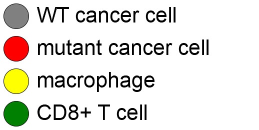
- WT cancer cells: Proliferate and release a signal that will stimulate an immune response. Cancer cells can transform into mutant cancer cells. Dead cells release debris. Damage increases apoptotic cell death.
- Mutant cancer cells: Proliferate but release less of the signal, as a model of immune evasion. Dead cells release debris. Damage increases apoptotic cell death.
- Macrophages: Chemotax towards the tumor signal and debris, and release a pro-inflammatory signal. They phagocytose dead cells.
- CD8+ T cells: Chemotax towards the pro-inflammatory signal and cause damage to tumor cells. As a model of immune evasion, CD8+ T cells can damage WT cancer cells faster than mutant cancer cells.
We will use the following diffusing factors:
- Tumor signal: Released by WT and mutant cells at different rates. We’ll fix a 1 min\(^{-1}\) decay rate and set the diffusion parameter to 10000 \(\mu m^2/\)min to give a 100 micron diffusion length scale.
- Pro-inflammatory signal: Released by macrophages. We’ll fix a 1 min\(^{-1}\) decay rate and set the diffusion parameter to 10000 \(\mu;m^2/\)min to give a 100 micron diffusion length scale.
- Debris: Released by dead cells. We’ll fix a 0.01 min\(^{-1}\) decay rate and choose a diffusion coefficient of 1 \(\mu;m^2/\)min for a 10 micron diffusion length scale.
In particular, we won’t worry about oxygen or resources in this model. We can use Neumann (no flux) boundary conditions.
Getting started with a template project and the graphical model builder
The PhysiCell Model Builder was developed by Randy Heiland and undergraduate researchers at Indiana University to help ease the creation of PhysiCell models, with a focus on generating correct XML configuration files that define the diffusing substrates and cell definitions. Here, we assume that you have cloned (or downloaded) the repository adjacent to your PhysiCell repository. (So that the path to PMB from PhysiCell’s root directory is ../PhysiCell-model-builder/).
Let’s start a new project (starting with the template project) from a command prompt or shell in the PhysiCell directory, and then open the model builder.
make template
make
python ../PhysiCell-model-builder/bin/pmb.py
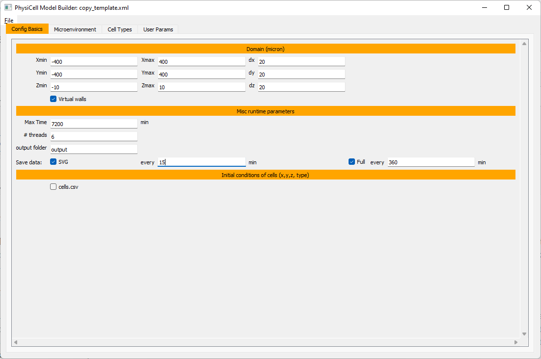
Setting up the domain
Let’s use a [-400,400] x [-400,400] 2D domain, with “virtual walls” enabled (so cells stay in the domain). We’ll run for 5760 minutes (4 days), saving SVG outputs every 15 minutes.
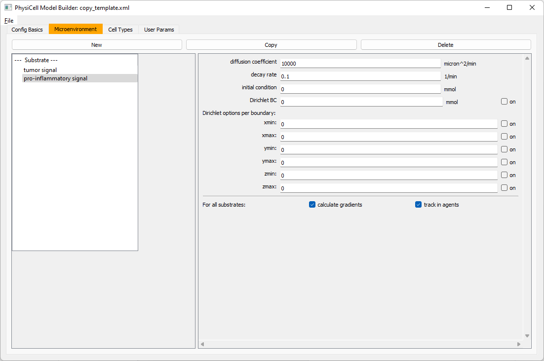
Setting up diffusing substrates
Move to the microenvironment tab. Click on substrate and rename it to tumor signal . Set the decay rate to 0.1 and diffusion parameter to 10000. Uncheck the Dirichlet condition box so that it’s a zero-flux (Neumann) boundary condition.
 Now, select
 tumor signal in the lefthand column, click copy, and rename the new substrate (substrate01) to pro-inflammatory signal with the same parameters.
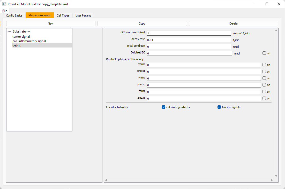
Then, copy this substrate one more time, and rename it from name debris. Set its decay rate to 0.01, and its diffusion parameter to 1.
Let’s save our work before continuing. Go to File, Save as, and save it as PhysiCell_settings.xml in your config file. (Go ahead and overwrite.)
If model builder crashes, you can reopen it, then go to File, Open, and select this file to continue editing.
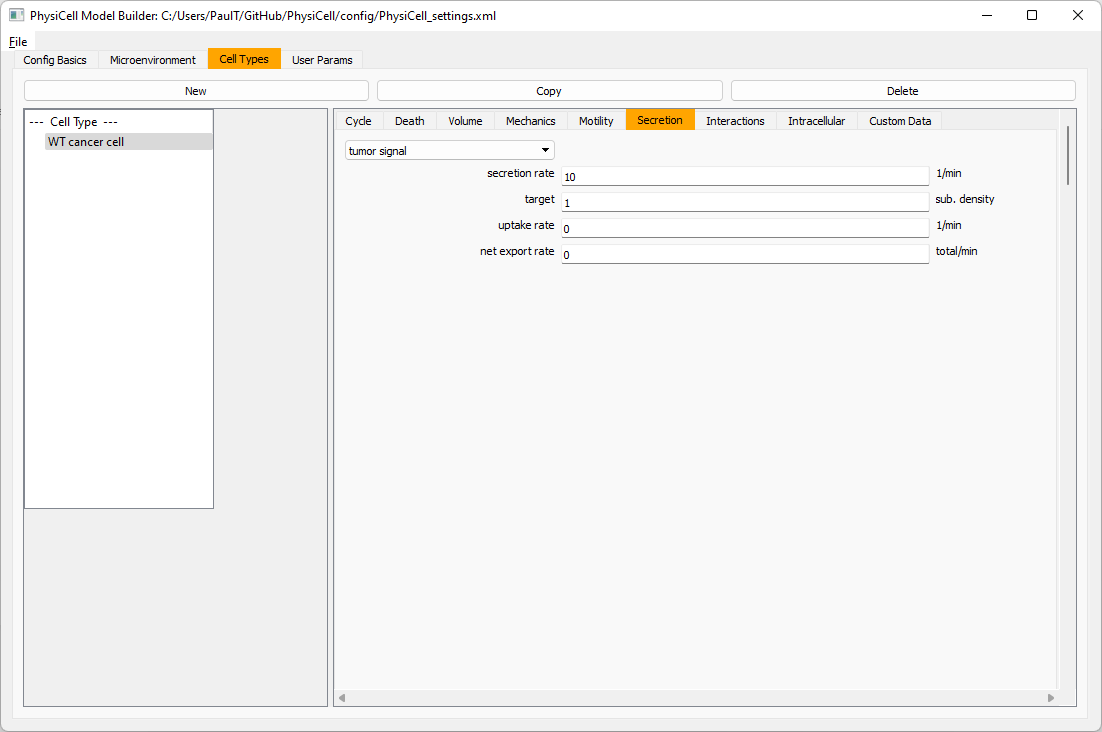
Setting up the WT cancer cells
Move to the cell types tab. Click on the default cell type on the left side, and rename it to WT cancer cell. Leave most of the parameter values at their defaults. Move to the secretion sub-tab (in phenotype). From the drop-down menu, select tumor signal. Let’s set a high secretion rate of 10.
We’ll need to set WT cells as able to mutate, but before that, the model builder needs to “know” about that cell type. So, let’s move on to the next cell type for now.
Setting up mutant tumor cells
Click the WT cancer cell in the left column, and click copy. Rename this cell type (for me, it’s cell_def03) to mutant cancer cell. Click the secretion sub-tab, and set its secretion rate of tumor signal lower to 0.1.
Set the WT mutation rate
Now that both cell types are in the simulation, we can set up mutation. Let’s suppose the mean time to a mutation is 10000 minutes, or a rate of 0.0001 min\(^{-1}\).
Click the WT cancer cell in the left column to select it. Go to the interactions tab. Go down to transformation rate, and choose mutant cancer cell from the drop-down menu. Set its rate to 0.0001.

Create macrophages
Now click on the WT cancer cell type in the left column, and click copy to create a new cell type. Click on the new type (for me cell_def04) and rename it to macrophage.
Click on cycle and change to a live cells and change from a duration representation to a transition rate representation. Keep its cycling rate at 0.
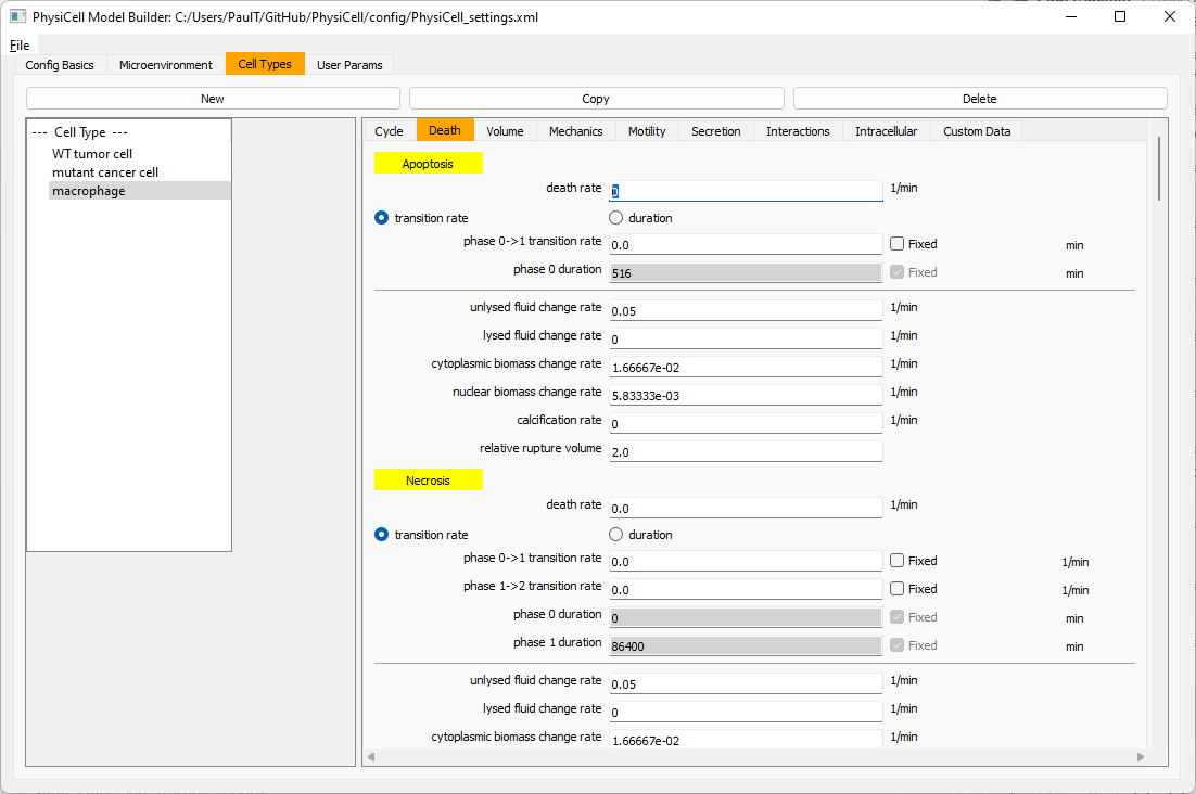
Go to death and change from duration to transition rate for both apoptosis and necrosis, and keep the death rates at 0.0
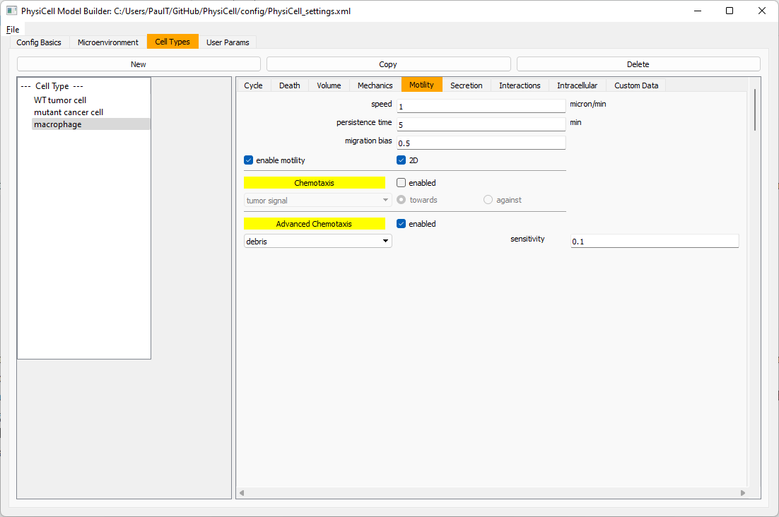
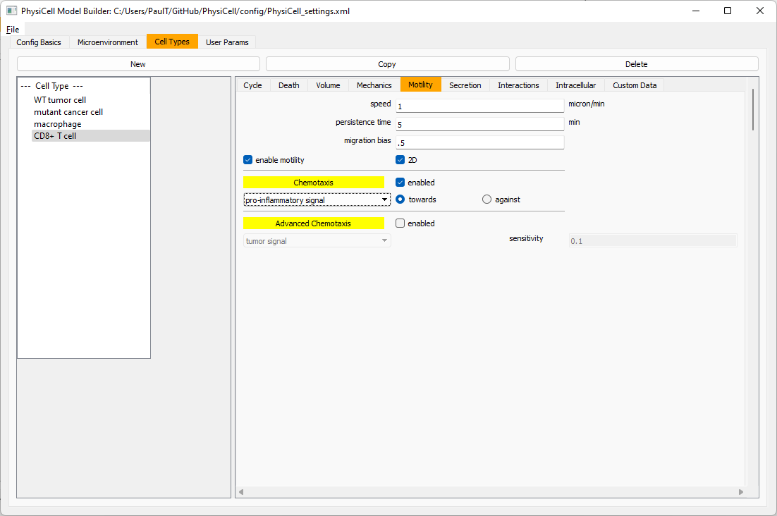
Now, go to the motility tab. Set the speed to 1 \(\mu m/\)min, persistence time to 5 min, and migration bias to 0.5. Be sure to enable motility. Then, enable advanced motility. Choose tumor signal from the drop-down and set its sensitivity to 1.0. Then choose debris from the drop-down and set its sensitivity to 0.1
Now, let’s make sure it secretes pro-inflammatory signal. Go to the secretion tab. Choose tumor signal from the drop-down, and make sure its secretion rate is 0. Then choose pro-inflammatory signal from the drop-down, set its secretion rate to 100, and its target value to 1.

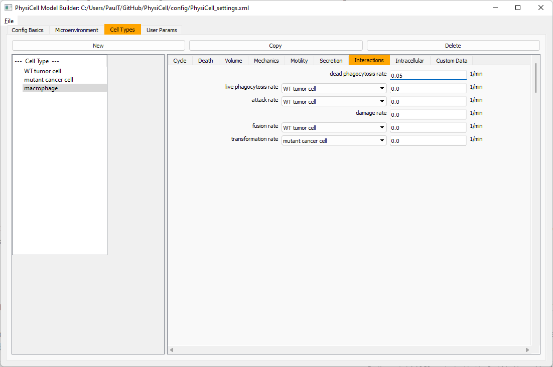
Lastly, let’s set macrophages up to phagocytose dead cells. Go to the interactions tab. Set the dead phagocytosis rate to 0.05 (so that the mean contact time to wait to eat a dead cell is 1/0.05 = 20 minutes). This would be a good time to save your work.
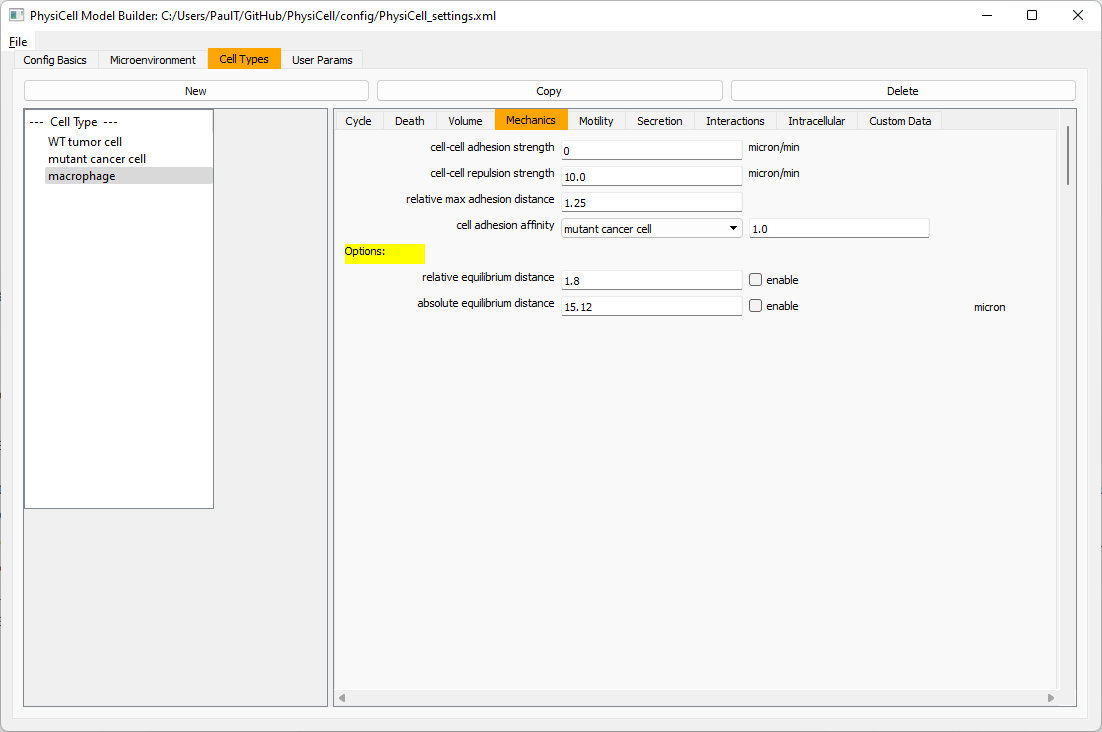
Macrophages probably shouldn’t be adhesive. So go to the mechanics sub-tab, and set the cell-cell adhesion strength to 0.0.
Create CD8+ T cells
Select macrophage on the left column, and choose copy. Rename the new cell type to CD8+ T cell. Go to the secretion sub-tab and make sure to set the secretion rate of pro-inflammatory signal to 0.0.
Now, let’s use simpler chemotaxis for these towards pro-inflammatory signal. Go to the motility tab. Uncheck advanced chemotaxis and check chemotaxis. Choose pro-inflammatory signal from the drop-down, with the towards option.
Lastly, let’s set these cells to attack WT and tumor cells. Go to the interactions tab. Set the dead phagocytosis rate to 0.
Now, let’s work on attack. Set the damage rate to 1.0. Near attack rate, choose WT tumor cell from the drop-down, and set its attack rate to 10 (so it attacks during any 0.1 minute interval). Then choose mutant tumor cell from the drop-down, and set its attack rate to 1 (as a model of immune evasion, where they are less likely to attack a non-WT tumor cell).

Set the initial cell conditions
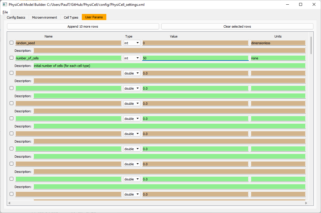
Go to the user params tab. On number of cells, choose 50. It will randomly place 50 of each cell type at the start of the simulation.
That’s all! Go to File and save (or save as), and overwrite config/PhysiCell_settings.xml. Then close the model builder.
Testing the model
Go into the PhysiCell directory. Since you already compiled, just run your model (which will use PhysiCell_settings.xml that you just saved to the config directory). For Linux or MacOS (or similar Unix-like systems):
./project
Windows users would type project without the ./ at the front.
Take a look at your SVG outputs in the output directory. You might consider making an animated gif (make gif) or a movie:
make jpeg && make movie
Here’s what we have.
 |
Promising! But we still need to write a little C++ so that damage kills tumor cells, and so that dead tumor cells release debris. (And we could stand to “anchor” tumor cells to ECM so they don’t get pushed around by the immune cells, but that’s a post for another day!)
Customizing the WT and mutant tumor cells with phenotype functions
First, open custom.h in the custom_modules directory, and declare a function for tumor phenotype:
void tumor_phenotype_function( Cell* pCell, Phenotype& phenotype, double dt );
Now, let’s open custom.cpp to write this function at the bottom. Here’s what we’ll do:
- If dead, set rate of debris release to 1.0 and return.
- Otherwise, we’ll set damage-based apoptosis.
- Get the base apoptosis rate
- Get the current damage
- Use a Hill response function with a half-max of 36, max apoptosis rate of 0.05 min\(^{-1}\), and a hill power of 2.0
Here’s the code:
void tumor_phenotype_function( Cell* pCell, Phenotype& phenotype, double dt )
{
   // find my cell definition
   static Cell_Definition* pCD = find_cell_definition( pCell->type_name );

   // find the index of debris in the environment
   static int nDebris = microenvironment.find_density_index( "debris" );
   static int nTS = microenvironment.find_density_index( "tumor signal" );

   // if dead: release debris. stop releasing tumor signal
   if( phenotype.death.dead == true )
   {
      phenotype.secretion.secretion_rates[nDebris] = 1;
      phenotype.secretion.saturation_densities[nDebris] = 1;

      phenotype.secretion.secretion_rates[nTS] = 0;

      // last time I'll execute this function (special optional trick)
      pCell->functions.update_phenotype = NULL;
      return;
   }

   // damage increases death

   // find death model
   static int nApoptosis =
      phenotype.death.find_death_model_index( PhysiCell_constants::apoptosis_death_model );

   double signal = pCell->state.damage; // current damage
   double base_val = pCD->phenotype.death.rates[nApoptosis]; // base death rate (from cell def)
   double max_val = 0.05; // max death rate (at large damage)

   static double damage_halfmax = 36.0;
   double hill_power = 2.0;

   // evaluate Hill response function
   double hill = Hill_response_function( signal , damage_halfmax , hill_power );
   // set "dose-dependent" death rate
   phenotype.death.rates[nApoptosis] = base_val + (max_val-base_val)*hill;

   return;
}
Now, we need to make sure we apply these functions to tumor cell. Go to `create_cell_types` and look just before we display the cell definitions. We need to:
- Search for the WT tumor cell definition
- Set the update_phenotype function for that type to the tumor_phenotype_function we just wrote
- Repeat for the mutant tumor cell type.
Here’s the code:
...
   /*
      Put any modifications to individual cell definitions here.

      This is a good place to set custom functions.
   */

   cell_defaults.functions.update_phenotype = phenotype_function;
   cell_defaults.functions.custom_cell_rule = custom_function;
   cell_defaults.functions.contact_function = contact_function;

   Cell_Definition* pCD = find_cell_definition( "WT cancer cell");
   pCD->functions.update_phenotype = tumor_phenotype_function;

   pCD = find_cell_definition( "mutant cancer cell");
   pCD->functions.update_phenotype = tumor_phenotype_function;

   /*
      This builds the map of cell definitions and summarizes the setup.
   */

   display_cell_definitions( std::cout );
   return;
}
That’s it! Let’s recompile and run!
make && ./project
And here’s the final movie.
|
Much better! Now the
Coming up next!
We will use the signal and behavior dictionaries to help us easily write C++ functions to modulate the tumor and immune cell behaviors.
Once ready, this will be posted at http://www.mathcancer.org/blog/introducing-cell-signal-and-behavior-dictionaries/.
PhysiCell Tools : python-loader
The newest tool for PhysiCell provides an easy way to load your PhysiCell output data into python for analysis. This builds upon previous work on loading data into MATLAB. A post on that tool can be found at:
http://www.mathcancer.org/blog/working-with-physicell-snapshots-in-matlab/.
PhysiCell stores output data as a MultiCell Digital Snapshot (MultiCellDS) that consists of several files for each time step and is probably stored in your ./output directory. pyMCDS is a python object that is initialized with the .xml file
What you’ll need
- python-loader, available on GitHub at
- Python 3.x, recommended distribution available at
- A number of Python packages, included in anaconda or available through pip
- NumPy
- pandas
- scipy
- Some PhysiCell data, probably in your ./output directory
Anatomy of a MultiCell Digital Snapshot
Each time PhysiCell’s internal time tracker passes a time step where data is to be saved, it generates a number of files of various types. Each of these files will have a number at the end that indicates where it belongs in the sequence of outputs. All of the files from the first round of output will end in 00000000.* and the second round will be 00000001.* and so on. Let’s say we’re interested in a set of output from partway through the run, the 88th set of output files. The files we care about most from this set consists of:
- output00000087.xml: This file is the main organizer of the data. It contains an overview of the data stored in the MultiCellDS as well as some actual data including:
- Metadata about the time and runtime for the current time step
- Coordinates for the computational domain
- Parameters for diffusing substrates in the microenvironment
- Column labels for the cell data
- File names for the files that contain microenvironment and cell data at this time step
- output00000087_microenvironment0.mat: This is a MATLAB matrix file that contains all of the data about the microenvironment at this time step
- output00000087_cells_physicell.mat: This is a MATLAB matrix file that contains all of the tracked information about the individual cells in the model. It tells us things like the cells’ position, volume, secretion, cell cycle status, and user-defined cell parameters.
Setup
Using pyMCDS
From the appropriate file in your PhysiCell directory, wherever pyMCDS.py lives, you can use the data loader in your own scripts or in an interactive session. To start you have to import the pyMCDS class
from pyMCDS import pyMCDS
Loading the data
Data is loaded into python from the MultiCellDS by initializing the pyMCDS object. The initialization function for pyMCDS takes one required and one optional argument.
__init__(xml_file, [output_path = '.'])
    '''
    xml_file : string
        String containing the name of the output xml file
    output_path :
        String containing the path (relative or absolute) to the directory
        where PhysiCell output files are stored
    '''
We are interested in reading output00000087.xml that lives in ~/path/to/PhysiCell/output (don’t worry Windows paths work too). We would initialize our pyMCDS object using those names and the actual data would be stored in a member dictionary called data.
mcds = pyMCDS('output00000087.xml', '~/path/to/PhysiCell/output')
# Now our data lives in:
mcds.data
We’ve tried to keep everything organized inside of this dictionary but let’s take a look at what we actually have in here. Of course in real output, there will probably not be a chemical named my_chemical, this is simply there to illustrate how multiple chemicals are handled.

The data member dictionary is a dictionary of dictionaries whose child dictionaries can be accessed through normal python dictionary syntax.
mcds.data['metadata']
mcds.data['continuum_variables']['my_chemical']
Each of these subdictionaries contains data, we will take a look at exactly what that data is and how it can be accessed in the following sections.
Metadata
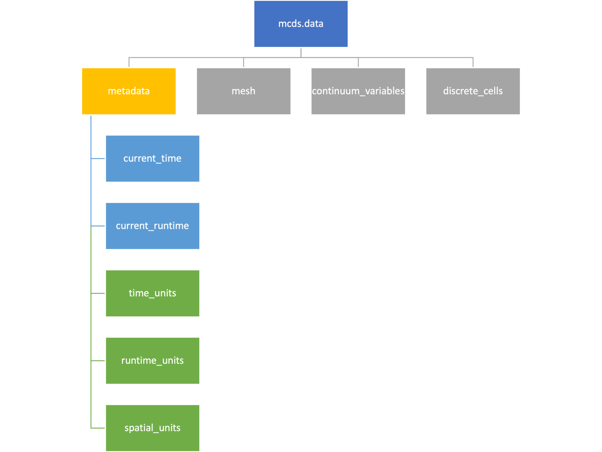
The metadata dictionary contains information about the time of the simulation as well as units for both times and space. Here and in later sections blue boxes indicate scalars and green boxes indicate strings. We can access each of these things using normal dictionary syntax. We’ve also got access to a helper function get_time() for the common operation of retrieving the simulation time.
>>> mcds.data['metadata']['time_units']
'min'
>>> mcds.get_time()
5220.0
Mesh
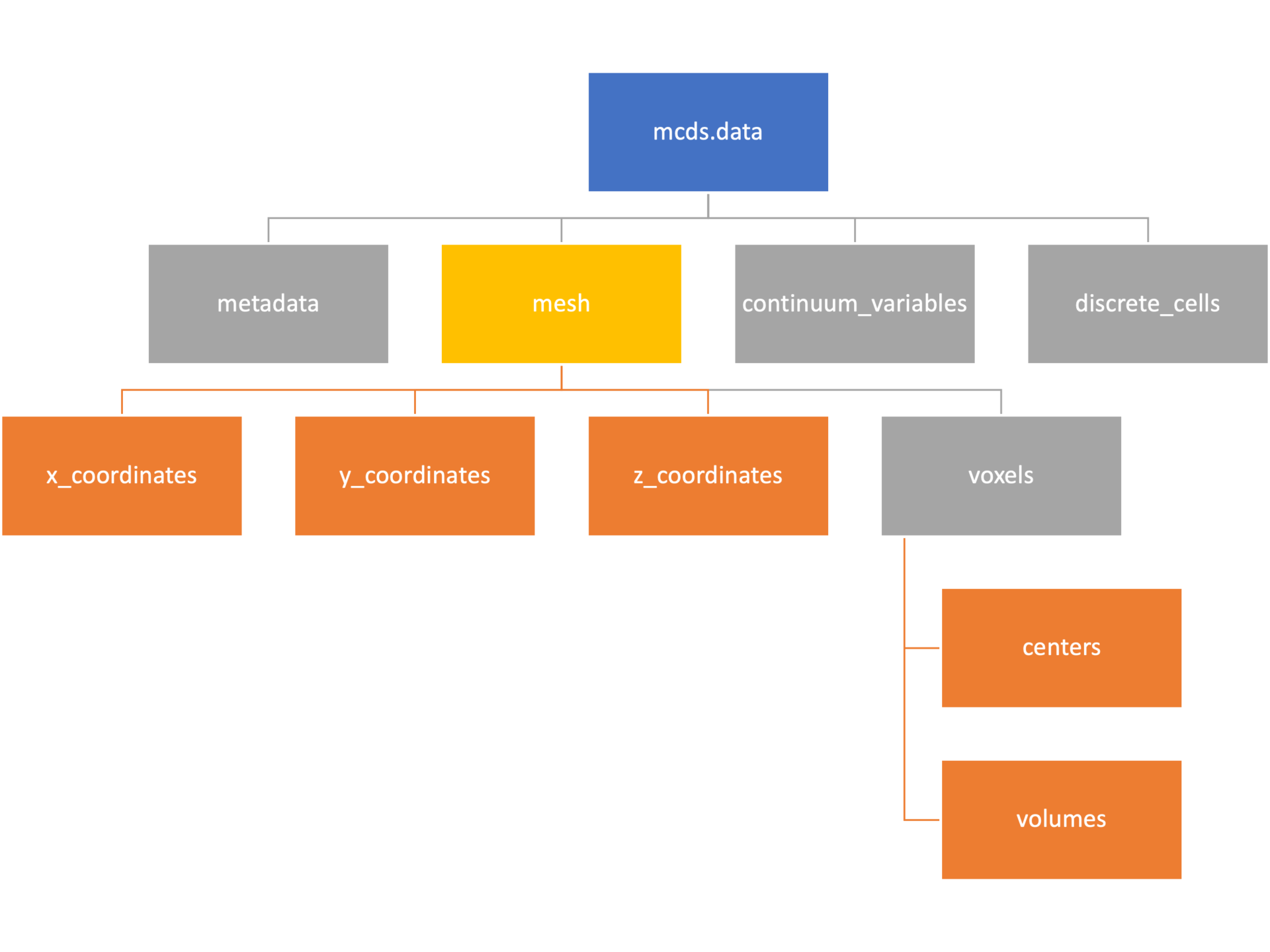
The mesh dictionary has a lot more going on than the metadata dictionary. It contains three numpy arrays, indicated by orange boxes, as well as another dictionary. The three arrays contain \(x\), \(y\) and \(z\) coordinates for the centers of the voxels that constiture the computational domain in a meshgrid format. This means that each of those arrays is tensors of rank three. Together they identify the coordinates of each possible point in the space.
In contrast, the arrays in the voxel dictionary are stored linearly. If we know that we care about voxel number 42, we want to use the stuff in the voxels dictionary. If we want to make a contour plot, we want to use the x_coordinates, y_coordinates, and z_coordinates arrays.
# We can extract one of the meshgrid arrays as a numpy array
>>> y_coords = mcds.data['mesh']['y_coordinates']
>>> y_coords.shape
(75, 75, 75)
>>> y_coords[0, 0, :4]
array([-740., -740., -740., -740.])

# We can also extract the array of voxel centers
>>> centers = mcds.data['mesh']['voxels']['centers']
>>> centers.shape
(3, 421875)
>>> centers[:, :4]
array([[-740., -720., -700., -680.],
       [-740., -740., -740., -740.],
       [-740., -740., -740., -740.]])

# We have a handy function to quickly extract the components of the full meshgrid
>>> xx, yy, zz = mcds.get_mesh()
>>> yy.shape
(75, 75, 75)
>>> yy[0, 0, :4]
array([-740., -740., -740., -740.])

# We can also use this to return the meshgrid describing an x, y plane
>>> xx, yy = mcds.get_2D_mesh()
>>> yy.shape
(75, 75)
Continuum variables
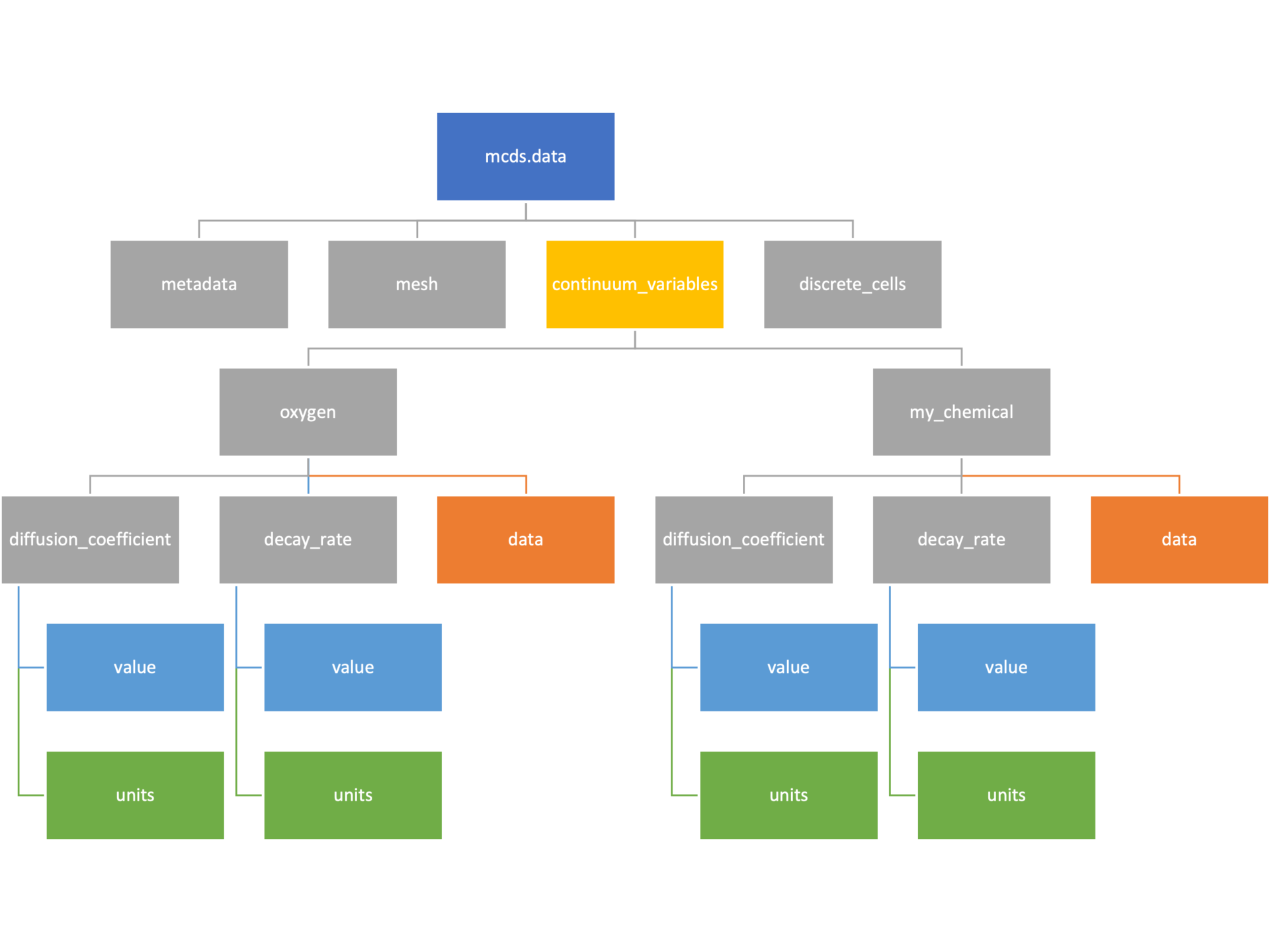
The continuum_variables dictionary is the most complicated of the four. It contains subdictionaries that we access using the names of each of the chemicals in the microenvironment. In our toy example above, these are oxygen and my_chemical. If our model tracked diffusing oxygen, VEGF, and glucose, then the continuum_variables dictionary would contain a subdirectory for each of them.
For a particular chemical species in the microenvironment we have two more dictionaries called decay_rate and diffusion_coefficient, and a numpy array called data. The diffusion and decay dictionaries each complete the value stored as a scalar and the unit stored as a string. The numpy array contains the concentrations of the chemical in each voxel at this time and is the same shape as the meshgrids of the computational domain stored in the .data[‘mesh’] arrays.
# we need to know the names of the substrates to work with
# this data. We have a function to help us find them.
>>> mcds.get_substrate_names()
['oxygen', 'my_chemical']

# The diffusable chemical dictionaries are messy
# if we need to do a lot with them it might be easier
# to put them into their own instance
>>> oxy_dict = mcds.data['continuum_variables']['oxygen']
>>> oxy_dict['decay_rate']
{'value': 0.1, 'units': '1/min'}

# What we care about most is probably the numpy
# array of concentrations
>>> oxy_conc = oxy_dict['data']
>>> oxy_conc.shape
(75, 75, 75)

# Alternatively, we can get the same array with a function
>>> oxy_conc2 = mcds.get_concentrations('oxygen')
>>> oxy_conc2.shape
(75, 75, 75)

# We can also get the concentrations on a plane using the
# same function and supplying a z value to "slice through"
# note that right now the z_value must be an exact match
# for a plane of voxel centers, in the future we may add
# interpolation.
>>> oxy_plane = mcds.get_concentrations('oxygen', z_value=100.0)
>>> oxy_plane.shape
(75, 75)

# we can also find the concentration in a single voxel using the
# position of a point within that voxel. This will give us an
# array of all concentrations at that point.
>>> mcds.get_concentrations_at(x=0., y=550., z=0.)
array([17.94514446,  0.99113448])
Discrete Cells

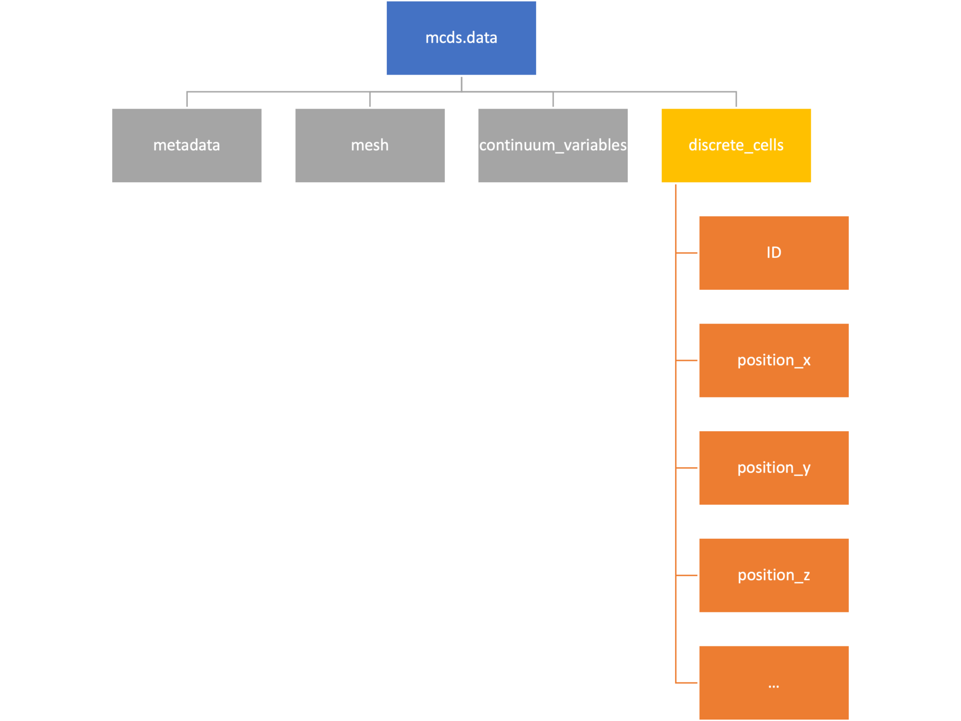
The discrete cells dictionary is relatively straightforward. It contains a number of numpy arrays that contain information regarding individual cells. These are all 1-dimensional arrays and each corresponds to one of the variables specified in the output*.xml file. With the default settings, these are:
- ID: unique integer that will identify the cell throughout its lifetime in the simulation
- position(_x, _y, _z): floating point positions for the cell in \(x\), \(y\), and \(z\) directions
- total_volume: total volume of the cell
- cell_type: integer label for the cell as used in PhysiCell
- cycle_model: integer label for the cell cycle model as used in PhysiCell
- current_phase: integer specification for which phase of the cycle model the cell is currently in
- elapsed_time_in_phase: time that cell has been in current phase of cell cycle model
- nuclear_volume: volume of cell nucleus
- cytoplasmic_volume: volume of cell cytoplasm
- fluid_fraction: proportion of the volume due to fliud
- calcified_fraction: proportion of volume consisting of calcified material
- orientation(_x, _y, _z): direction in which cell is pointing
- polarity:
- migration_speed: current speed of cell
- motility_vector(_x, _y, _z): current direction of movement of cell
- migration_bias: coefficient for stochastic movement (higher is “more deterministic”)
- motility_bias_direction(_x, _y, _z): direction of movement bias
- persistence_time: time in-between direction changes for cell
- motility_reserved:
# Extracting single variables is just like before
>>> cell_ids = mcds.data['discrete_cells']['ID']
>>> cell_ids.shape
(18595,)
>>> cell_ids[:4]
array([0., 1., 2., 3.])

# If we're clever we can extract 2D arrays
>>> cell_vec = np.zeros((cell_ids.shape[0], 3))
>>> vec_list = ['position_x', 'position_y', 'position_z']
>>> for i, lab in enumerate(vec_list):
...     cell_vec[:, i] = mcds.data['discrete_cells'][lab]
...
array([[ -69.72657128,  -39.02046405, -233.63178904],
       [ -69.84507464,  -22.71693265, -233.59277388],
       [ -69.84891462,   -6.04070516, -233.61816711],
       [ -69.845265  ,   10.80035554, -233.61667313]])

# We can get the list of all of the variables stored in this dictionary
>>> mcds.get_cell_variables()
['ID',
 'position_x',
 'position_y',
 'position_z',
 'total_volume',
 'cell_type',
 'cycle_model',
 'current_phase',
 'elapsed_time_in_phase',
 'nuclear_volume',
 'cytoplasmic_volume',
 'fluid_fraction',
 'calcified_fraction',
 'orientation_x',
 'orientation_y',
 'orientation_z',
 'polarity',
 'migration_speed',
 'motility_vector_x',
 'motility_vector_y',
 'motility_vector_z',
 'migration_bias',
 'motility_bias_direction_x',
 'motility_bias_direction_y',
 'motility_bias_direction_z',
 'persistence_time',
 'motility_reserved',
 'oncoprotein',
 'elastic_coefficient',
 'kill_rate',
 'attachment_lifetime',
 'attachment_rate']
# We can also get all of the cell data as a pandas DataFrame
>>> cell_df = mcds.get_cell_df()
>>> cell_df.head()
ID     position_x   position_y    position_z total_volume cell_type cycle_model ...
0.0   - 69.726571  - 39.020464  - 233.631789       2494.0       0.0         5.0 ...
1.0   - 69.845075  - 22.716933  - 233.592774       2494.0       0.0         5.0 ...
2.0   - 69.848915  - 6.040705   - 233.618167       2494.0       0.0         5.0 ...
3.0   - 69.845265    10.800356  - 233.616673       2494.0       0.0         5.0 ...
4.0   - 69.828161    27.324530  - 233.631579       2494.0       0.0         5.0 ...

# if we want to we can also get just the subset of cells that
# are in a specific voxel
>>> vox_df = mcds.get_cell_df_at(x=0.0, y=550.0, z=0.0)
>>> vox_df.iloc[:, :5]
             ID  position_x  position_y  position_z  total_volume
26718  228761.0    6.623617  536.709341   -1.282934   2454.814507
52736  270274.0   -7.990034  538.184921    9.648955   1523.386488
Examples
These examples will not be made using our toy dataset described above but will instead be made using a single timepoint dataset that can be found at:
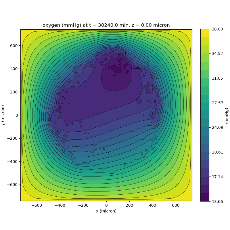
Substrate contour plot
One of the big advantages of working with PhysiCell data in python is that we have access to its plotting tools. For the sake of example let’s plot the partial pressure of oxygen throughout the computational domain along the \(z = 0\) plane. Once we’ve loaded our data by initializing a pyMCDS object, we can work entirely within python to produce the plot.
from pyMCDS import pyMCDS
import numpy as np
import matplotlib.pyplot as plt

# load data
mcds = pyMCDS('output00003696.xml', '../output')

# Set our z plane and get our substrate values along it
z_val = 0.00
plane_oxy = mcds.get_concentrations('oxygen', z_slice=z_val)

# Get the 2D mesh for contour plotting
xx, yy = mcds.get_mesh()

# We want to be able to control the number of contour levels so we
# need to do a little set up
num_levels = 21
min_conc = plane_oxy.min()
max_conc = plane_oxy.max()
my_levels = np.linspace(min_conc, max_conc, num_levels)

# set up the figure area and add data layers
fig, ax = plt.subplot()
cs = ax.contourf(xx, yy, plane_oxy, levels=my_levels)
ax.contour(xx, yy, plane_oxy, color='black', levels = my_levels,
           linewidths=0.5)

# Now we need to add our color bar
cbar1 = fig.colorbar(cs, shrink=0.75)
cbar1.set_label('mmHg')

# Let's put the time in to make these look nice
ax.set_aspect('equal')
ax.set_xlabel('x (micron)')
ax.set_ylabel('y (micron)')
ax.set_title('oxygen (mmHg) at t = {:.1f} {:s}, z = {:.2f} {:s}'.format(
                                        mcds.get_time(),
                                        mcds.data['metadata']['time_units'],
                                        z_val,
                                        mcds.data['metadata']['spatial_units'])

plt.show()
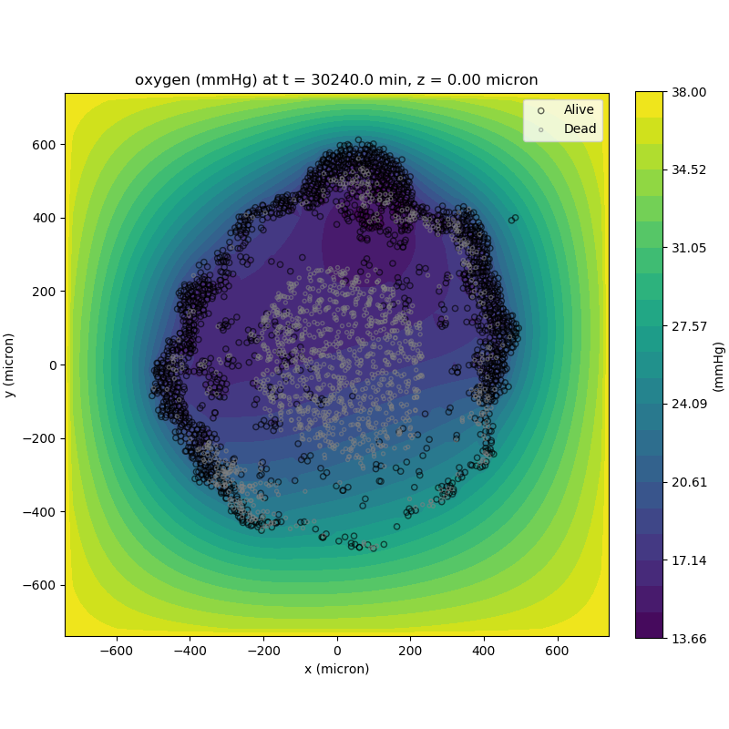
Adding a cells layer
We can also use pandas to do fairly complex selections of cells to add to our plots. Below we use pandas and the previous plot to add a cells layer.
from pyMCDS import pyMCDS
import numpy as np
import matplotlib.pyplot as plt

# load data
mcds = pyMCDS('output00003696.xml', '../output')

# Set our z plane and get our substrate values along it
z_val = 0.00
plane_oxy = mcds.get_concentrations('oxygen', z_slice=z_val)

# Get the 2D mesh for contour plotting
xx, yy = mcds.get_mesh()

# We want to be able to control the number of contour levels so we
# need to do a little set up
num_levels = 21
min_conc = plane_oxy.min()
max_conc = plane_oxy.max()
my_levels = np.linspace(min_conc, max_conc, num_levels)

# get our cells data and figure out which cells are in the plane
cell_df = mcds.get_cell_df()
ds = mcds.get_mesh_spacing()
inside_plane = (cell_df['position_z'] < z_val + ds) \ & (cell_df['position_z'] > z_val - ds)
plane_cells = cell_df[inside_plane]

# We're going to plot two types of cells and we want it to look nice
colors = ['black', 'grey']
sizes = [20, 8]
labels = ['Alive', 'Dead']

# set up the figure area and add microenvironment layer
fig, ax = plt.subplot()
cs = ax.contourf(xx, yy, plane_oxy, levels=my_levels)

# get our cells of interest
# alive_cells = plane_cells[plane_cells['cycle_model'] < 6]
# dead_cells = plane_cells[plane_cells['cycle_model'] > 6]
# -- for newer versions of PhysiCell
alive_cells = plane_cells[plane_cells['cycle_model'] < 100]
dead_cells = plane_cells[plane_cells['cycle_model'] >= 100]

# plot the cell layer
for i, plot_cells in enumerate((alive_cells, dead_cells)):
    ax.scatter(plot_cells['position_x'].values,
            plot_cells['position_y'].values,
            facecolor='none',
            edgecolors=colors[i],
            alpha=0.6,
            s=sizes[i],
            label=labels[i])

# Now we need to add our color bar
cbar1 = fig.colorbar(cs, shrink=0.75)
cbar1.set_label('mmHg')

# Let's put the time in to make these look nice
ax.set_aspect('equal')
ax.set_xlabel('x (micron)')
ax.set_ylabel('y (micron)')
ax.set_title('oxygen (mmHg) at t = {:.1f} {:s}, z = {:.2f} {:s}'.format(
                                        mcds.get_time(),
                                        mcds.data['metadata']['time_units'],
                                        z_val,
                                        mcds.data['metadata']['spatial_units'])
ax.legend(loc='upper right')

plt.show()
Future Direction
The first extension of this project will be timeseries functionality. This will provide similar data loading functionality but for a time series of MultiCell Digital Snapshots instead of simply one point in time.
PhysiCell Tools : PhysiCell-povwriter
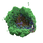
As PhysiCell matures, we are starting to turn our attention to better training materials and an ecosystem of open source PhysiCell tools. PhysiCell-povwriter is is designed to help transform your 3-D simulation results into 3-D visualizations like this one:
PhysiCell-povwriter transforms simulation snapshots into 3-D scenes that can be rendered into still images using POV-ray: an open source software package that uses raytracing to mimic the path of light from a source of illumination to a single viewpoint (a camera or an eye). The result is a beautifully rendered scene (at any resolution you choose) with very nice shading and lighting.
If you repeat this on many simulation snapshots, you can create an animation of your work.
What you’ll need
This workflow is entirely based on open source software:
- 3-D simulation data (likely stored in ./output from your project)
- PhysiCell-povwriter, available on GitHub at
- POV-ray, available at
- ImageMagick (optional, for image file conversions)
- mencoder (optional, for making compressed movies)
Setup
Building PhysiCell-povwriter
After you clone PhysiCell-povwriter or download its source from a release, you’ll need to compile it. In the project’s root directory, compile the project by:
make
(If you need to set up a C++ PhysiCell development environment, click here for OSX or here for Windows.)
Next, copy povwriter (povwriter.exe in Windows) to either the root directory of your PhysiCell project, or somewhere in your path. Copy ./config/povwriter-settings.xml to the ./config directory of your PhysiCell project.
Editing resolutions in POV-ray
PhysiCell-povwriter is intended for creating “square” images, but POV-ray does not have any pre-created square rendering resolutions out-of-the-box. However, this is straightforward to fix.
- Open POV-Ray
- Go to the “tools” menu and select “edit resolution INI file”
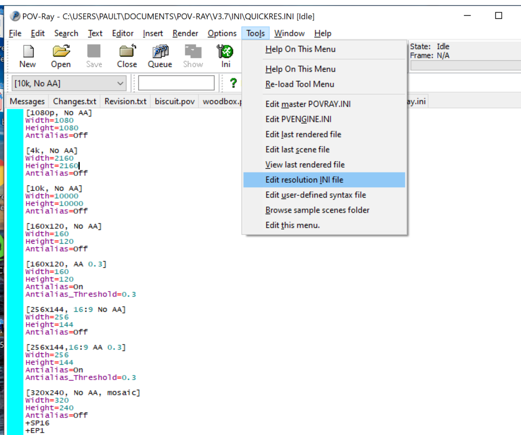
- At the top of the INI file (which opens for editing in POV-ray), make a new profile:
[1080x1080, AA]
Width=480
Height=480
Antialias=On
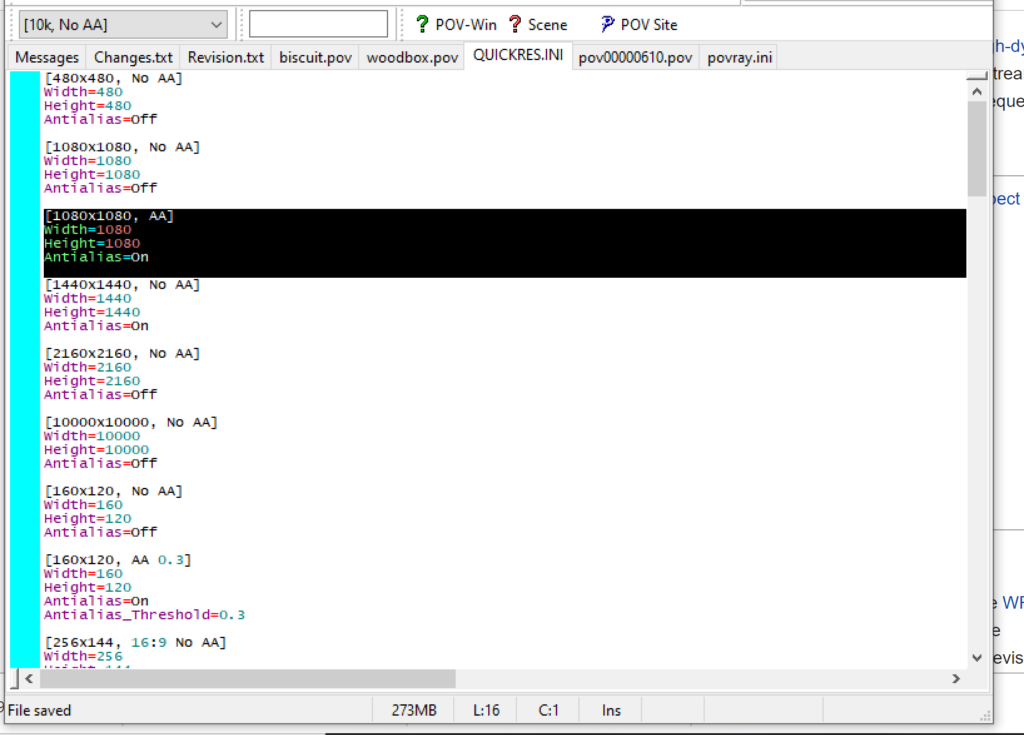
- Make similar profiles (with unique names) to suit your preferences. I suggest one at 480×480 (as a fast preview), another at 2160×2160, and another at 5000×5000 (because they will be absurdly high resolution). For example:
[2160x2160 no AA]
Width=2160
Height=2160
Antialias=Off
You can optionally make more profiles with antialiasing on (which provides some smoothing for areas of high detail), but you’re probably better off just rendering without antialiasing at higher resolutions and the scaling the image down as needed. Also, rendering without antialiasing will be faster.
- Once done making profiles, save and exit POV-Ray.
- The next time you open POV-Ray, your new resolution profiles will be available in the lefthand dropdown box.


Configuring PhysiCell-povwriter
Once you have copied povwriter-settings.xml to your project’s config file, open it in a text editor. Below, we’ll show the different settings.
Camera settings
<camera>
	<distance_from_origin units="micron">1500</distance_from_origin>
	<xy_angle>3.92699081699</xy_angle> <!-- 5*pi/4 -->
	<yz_angle>1.0471975512</yz_angle> <!-- pi/3 -->
</camera>
For simplicity, PhysiCell-POVray (currently) always aims the camera towards the origin (0,0,0), with “up” towards the positive z-axis. distance_from_origin sets how far the camera is placed from the origin. xy_angle sets the angle \(\theta\) from the positive x-axis in the xy-plane. yz_angle sets the angle \(\phi\) from the positive z-axis in the yz-plane. Both angles are in radians.
Options
<options>
	<use_standard_colors>true</use_standard_colors>
	<nuclear_offset units="micron">0.1</nuclear_offset>
	<cell_bound units="micron">750</cell_bound>
	<threads>8</threads>
</options>
use_standard_colors (if set to true) uses a built-in “paint-by-numbers” color scheme, where each cell type (identified with an integer) gets XML-defined colors for live, apoptotic, and dead cells. More on this below. If use_standard_colors is set to false, then PhysiCell-povwriter uses the my_pigment_and_finish_function in ./custom_modules/povwriter.cpp to color cells.
The nuclear_offset is a small additional height given to nuclei when cropping to avoid visual artifacts when rendering (which can cause some “tearing” or “bleeding” between the rendered nucleus and cytoplasm). cell_bound is used for leaving some cells out of bound: any cell with |x|, |y|, or |z| exceeding cell_bound will not be rendered. threads is used for parallelizing on multicore processors; note that it only speeds up povwriter if you are converting multiple PhysiCell outputs to povray files.
Save
<save> <!-- done -->
	<folder>output</folder> <!-- use . for root -->
	<filebase>output</filebase>
	<time_index>3696</time_index>
</save>
Use folder to tell PhysiCell-povwriter where the data files are stored. Use filebase to tell how the outputs are named. Typically, they have the form output########_cells_physicell.mat; in this case, the filebase is output. Lastly, use time_index to set the output number. For example if your file is output00000182_cells_physicell.mat, then filebase = output and time_index = 182.
Below, we’ll see how to specify ranges of indices at the command line, which would supersede the time_index given here in the XML.
Clipping planes
PhysiCell-povwriter uses clipping planes to help create cutaway views of the simulations. By default, 3 clipping planes are used to cut out an octant of the viewing area.
Recall that a plane can be defined by its normal vector n and a point p on the plane. With these, the plane can be defined as all points x satisfying
\[ \left( \vec{x} -\vec{p} \right) \cdot \vec{n} = 0 \]
These are then written out as a plane equation
\[ a x + by + cz + d = 0, \]
where
\[ (a,b,c) = \vec{n} \hspace{.5in} \textrm{ and } \hspace{0.5in} d = \: – \vec{n} \cdot \vec{p}. \]
As of Version 1.0.0, we are having some difficulties with clipping planes that do not pass through the origin (0,0,0), for which \( d = 0 \).
In the config file, these planes are written as \( (a,b,c,d) \):
<clipping_planes> <!-- done -->
	<clipping_plane>0,-1,0,0</clipping_plane>
	<clipping_plane>-1,0,0,0</clipping_plane>
	<clipping_plane>0,0,1,0</clipping_plane>
</clipping_planes>
Note that cells “behind” the plane (where \( ( \vec{x} – \vec{p} ) \cdot \vec{n} \le 0 \)) are rendered, and cells in “front” of the plane (where \( (\vec{x}-\vec{p}) \cdot \vec{n} > 0 \)) are not rendered. Cells that intersect the plane are partially rendered (using constructive geometry via union and intersection commands in POV-ray).
Cell color definitions
Within <cell_color_definitions>, you’ll find multiple <cell_colors> blocks, each of which defines the live, dead, and necrotic colors for a specific cell type (with the type ID indicated in the attribute). These colors are only applied if use_standard_colors is set to true in options. See above.
The live colors are given as two rgb (red,green,blue) colors for the cytoplasm and nucleus of live cells. Each element of this triple can range from 0 to 1, and not from 0 to 255 as in many raw image formats. Next, finish specifies ambient (how much highly-scattered background ambient light illuminates the cell), diffuse (how well light rays can illuminate the surface), and specular (how much of a shiny reflective splotch the cell gets).
See the POV-ray documentation for for information on the finish.
This is repeated to give the apoptotic and necrotic colors for the cell type.
<cell_colors type="0">
	<live>
		<cytoplasm>.25,1,.25</cytoplasm> <!-- red,green,blue -->
		<nuclear>0.03,0.125</nuclear>
		<finish>0.05,1,0.1</finish> <!-- ambient,diffuse,specular -->
	</live>
	<apoptotic>
		<cytoplasm>1,0,0</cytoplasm> <!-- red,green,blue -->
		<nuclear>0.125,0,0</nuclear>
		<finish>0.05,1,0.1</finish> <!-- ambient,diffuse,specular -->
	</apoptotic>
	<necrotic>
		<cytoplasm>1,0.5412,0.1490</cytoplasm> <!-- red,green,blue -->
		<nuclear>0.125,0.06765,0.018625</nuclear>
		<finish>0.01,0.5,0.1</finish> <!-- ambient,diffuse,specular -->
	</necrotic>
</cell_colors>
Use multiple cell_colors blocks (each with type corresponding to the integer cell type) to define the colors of multiple cell types.
Using PhysiCell-povwriter
Use by the XML configuration file alone
The simplest syntax:
physicell$ ./povwriter
(Windows users: povwriter or povwriter.exe) will process ./config/povwriter-settings.xml and convert the single indicated PhysiCell snapshot to a .pov file.
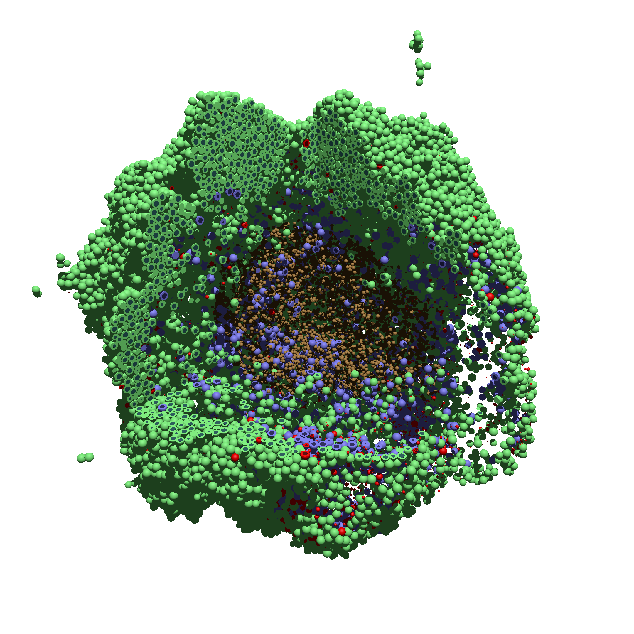
If you run POV-writer with the default configuration file in the povwriter structure (with the supplied sample data), it will render time index 3696 from the immunotherapy example in our 2018 PhysiCell Method Paper:
physicell$ ./povwriter

povwriter version 1.0.0
================================================================================

Copyright (c) Paul Macklin 2019, on behalf of the PhysiCell project
OSI License: BSD-3-Clause (see LICENSE.txt)

Usage:
================================================================================
povwriter : run povwriter with config file ./config/settings.xml

povwriter FILENAME.xml : run povwriter with config file FILENAME.xml

povwriter x:y:z : run povwriter on data in FOLDER with indices from x
to y in incremenets of z

Example: ./povwriter 0:2:10 processes files:
./FOLDER/FILEBASE00000000_physicell_cells.mat
./FOLDER/FILEBASE00000002_physicell_cells.mat
...
./FOLDER/FILEBASE00000010_physicell_cells.mat
(See the config file to set FOLDER and FILEBASE)

povwriter x1,...,xn : run povwriter on data in FOLDER with indices x1,...,xn

Example: ./povwriter 1,3,17 processes files:
./FOLDER/FILEBASE00000001_physicell_cells.mat
./FOLDER/FILEBASE00000003_physicell_cells.mat
./FOLDER/FILEBASE00000017_physicell_cells.mat
(Note that there are no spaces.)
(See the config file to set FOLDER and FILEBASE)

Code updates at https://github.com/PhysiCell-Tools/PhysiCell-povwriter

Tutorial & documentation at http://MathCancer.org/blog/povwriter
================================================================================

Using config file ./config/povwriter-settings.xml ...
Using standard coloring function ...
Found 3 clipping planes ...
Found 2 cell color definitions ...
Processing file ./output/output00003696_cells_physicell.mat...
Matrix size: 32 x 66978
Creating file pov00003696.pov for output ...
Writing 66978 cells ...
done!

Done processing all 1 files!
The result is a single POV-ray file (pov00003696.pov) in the root directory.
Now, open that file in POV-ray (double-click the file if you are in Windows), choose one of your resolutions in your lefthand dropdown (I’ll choose 2160×2160 no antialiasing), and click the green “run” button.
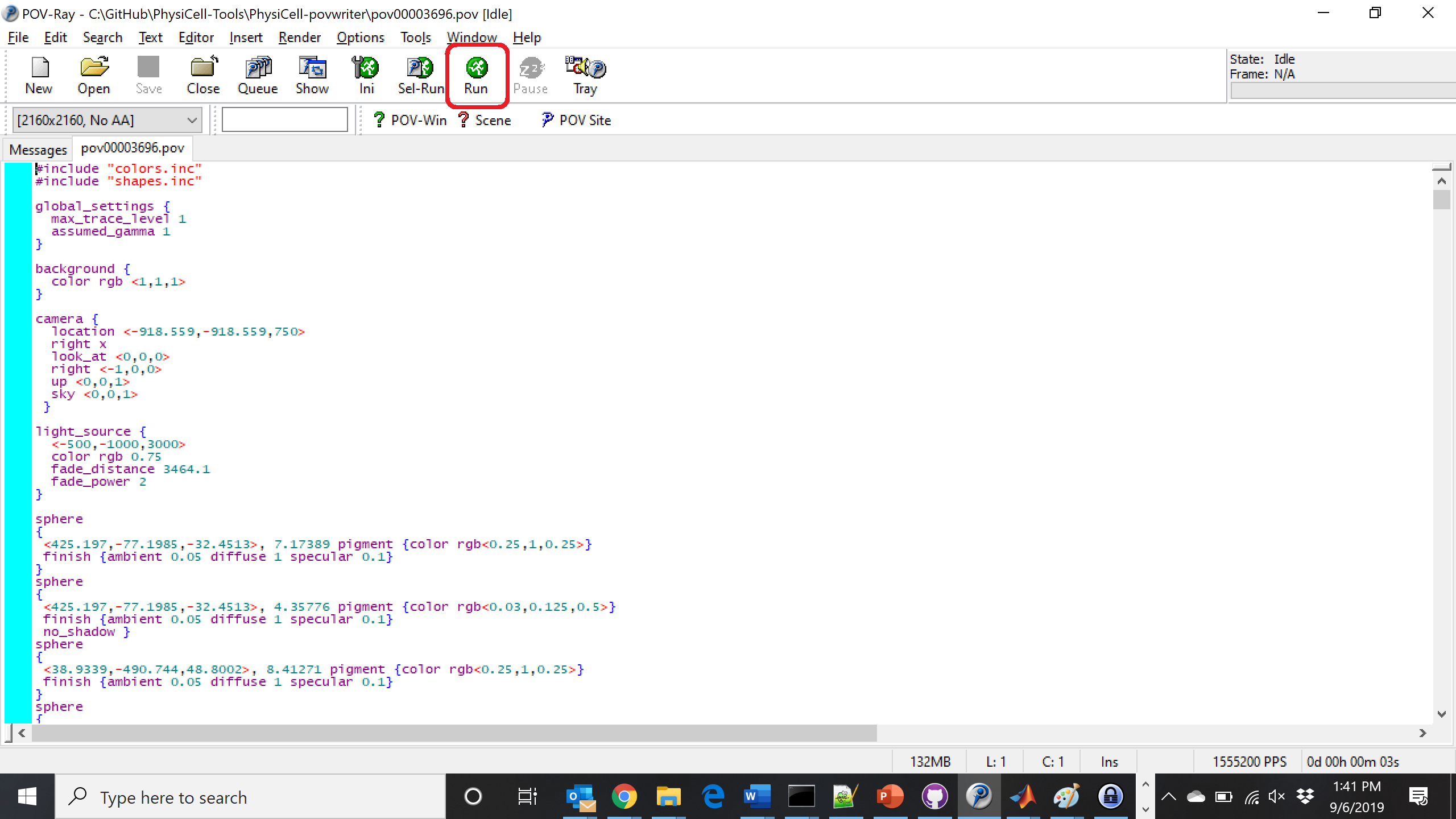
You can watch the image as it renders. The result should be a PNG file (named pov00003696.png) that looks like this:
Using command-line options to process multiple times (option #1)
Now, suppose we have more outputs to process. We still state most of the options in the XML file as above, but now we also supply a command-line argument in the form of start:interval:end. If you’re still in the povwriter project, note that we have some more sample data there. Let’s grab and process it:
physicell$ cd output
physicell$ unzip more_samples.zip
Archive: more_samples.zip
inflating: output00000000_cells_physicell.mat
inflating: output00000001_cells_physicell.mat
inflating: output00000250_cells_physicell.mat
inflating: output00000300_cells_physicell.mat
inflating: output00000500_cells_physicell.mat
inflating: output00000750_cells_physicell.mat
inflating: output00001000_cells_physicell.mat
inflating: output00001250_cells_physicell.mat
inflating: output00001500_cells_physicell.mat
inflating: output00001750_cells_physicell.mat
inflating: output00002000_cells_physicell.mat
inflating: output00002250_cells_physicell.mat
inflating: output00002500_cells_physicell.mat
inflating: output00002750_cells_physicell.mat
inflating: output00003000_cells_physicell.mat
inflating: output00003250_cells_physicell.mat
inflating: output00003500_cells_physicell.mat
inflating: output00003696_cells_physicell.mat

physicell$ ls

citation and license.txt
more_samples.zip
output00000000_cells_physicell.mat
output00000001_cells_physicell.mat
output00000250_cells_physicell.mat
output00000300_cells_physicell.mat
output00000500_cells_physicell.mat
output00000750_cells_physicell.mat
output00001000_cells_physicell.mat
output00001250_cells_physicell.mat
output00001500_cells_physicell.mat
output00001750_cells_physicell.mat
output00002000_cells_physicell.mat
output00002250_cells_physicell.mat
output00002500_cells_physicell.mat
output00002750_cells_physicell.mat
output00003000_cells_physicell.mat
output00003250_cells_physicell.mat
output00003500_cells_physicell.mat
output00003696.xml
output00003696_cells_physicell.mat
Let’s go back to the parent directory and run povwriter:
physicell$ ./povwriter 0:250:3500

povwriter version 1.0.0
================================================================================

Copyright (c) Paul Macklin 2019, on behalf of the PhysiCell project
OSI License: BSD-3-Clause (see LICENSE.txt)

Usage:
================================================================================
povwriter : run povwriter with config file ./config/settings.xml

povwriter FILENAME.xml : run povwriter with config file FILENAME.xml

povwriter x:y:z : run povwriter on data in FOLDER with indices from x
to y in incremenets of z

Example: ./povwriter 0:2:10 processes files:
./FOLDER/FILEBASE00000000_physicell_cells.mat
./FOLDER/FILEBASE00000002_physicell_cells.mat
...
./FOLDER/FILEBASE00000010_physicell_cells.mat
(See the config file to set FOLDER and FILEBASE)

povwriter x1,...,xn : run povwriter on data in FOLDER with indices x1,...,xn

Example: ./povwriter 1,3,17 processes files:
./FOLDER/FILEBASE00000001_physicell_cells.mat
./FOLDER/FILEBASE00000003_physicell_cells.mat
./FOLDER/FILEBASE00000017_physicell_cells.mat
(Note that there are no spaces.)
(See the config file to set FOLDER and FILEBASE)

Code updates at https://github.com/PhysiCell-Tools/PhysiCell-povwriter

Tutorial & documentation at http://MathCancer.org/blog/povwriter
================================================================================

Using config file ./config/povwriter-settings.xml ...
Using standard coloring function ...
Found 3 clipping planes ...
Found 2 cell color definitions ...
Matrix size: 32 x 18317
Processing file ./output/output00000000_cells_physicell.mat...
Creating file pov00000000.pov for output ...
Writing 18317 cells ...
Processing file ./output/output00002000_cells_physicell.mat...
Matrix size: 32 x 33551
Creating file pov00002000.pov for output ...
Writing 33551 cells ...
Processing file ./output/output00002500_cells_physicell.mat...
Matrix size: 32 x 43440
Creating file pov00002500.pov for output ...
Writing 43440 cells ...
Processing file ./output/output00001500_cells_physicell.mat...
Matrix size: 32 x 40267
Creating file pov00001500.pov for output ...
Writing 40267 cells ...
Processing file ./output/output00003000_cells_physicell.mat...
Matrix size: 32 x 56659
Creating file pov00003000.pov for output ...
Writing 56659 cells ...
Processing file ./output/output00001000_cells_physicell.mat...
Matrix size: 32 x 74057
Creating file pov00001000.pov for output ...
Writing 74057 cells ...
Processing file ./output/output00003500_cells_physicell.mat...
Matrix size: 32 x 66791
Creating file pov00003500.pov for output ...
Writing 66791 cells ...
Processing file ./output/output00000500_cells_physicell.mat...
Matrix size: 32 x 114316
Creating file pov00000500.pov for output ...
Writing 114316 cells ...
done!

Processing file ./output/output00000250_cells_physicell.mat...
Matrix size: 32 x 75352
Creating file pov00000250.pov for output ...
Writing 75352 cells ...
done!

Processing file ./output/output00002250_cells_physicell.mat...
Matrix size: 32 x 37959
Creating file pov00002250.pov for output ...
Writing 37959 cells ...
done!

Processing file ./output/output00001750_cells_physicell.mat...
Matrix size: 32 x 32358
Creating file pov00001750.pov for output ...
Writing 32358 cells ...
done!

Processing file ./output/output00002750_cells_physicell.mat...
Matrix size: 32 x 49658
Creating file pov00002750.pov for output ...
Writing 49658 cells ...
done!

Processing file ./output/output00003250_cells_physicell.mat...
Matrix size: 32 x 63546
Creating file pov00003250.pov for output ...
Writing 63546 cells ...
done!

done!

done!

done!

Processing file ./output/output00001250_cells_physicell.mat...
Matrix size: 32 x 54771
Creating file pov00001250.pov for output ...
Writing 54771 cells ...
done!

done!

done!

done!

Processing file ./output/output00000750_cells_physicell.mat...
Matrix size: 32 x 97642
Creating file pov00000750.pov for output ...
Writing 97642 cells ...
done!

done!

Done processing all 15 files!
Notice that the output appears a bit out of order. This is normal: povwriter is using 8 threads to process 8 files at the same time, and sending some output to the single screen. Since this is all happening simultaneously, it’s a bit jumbled (and non-sequential). Don’t panic. You should now have created pov00000000.pov, pov00000250.pov, … , pov00003500.pov.
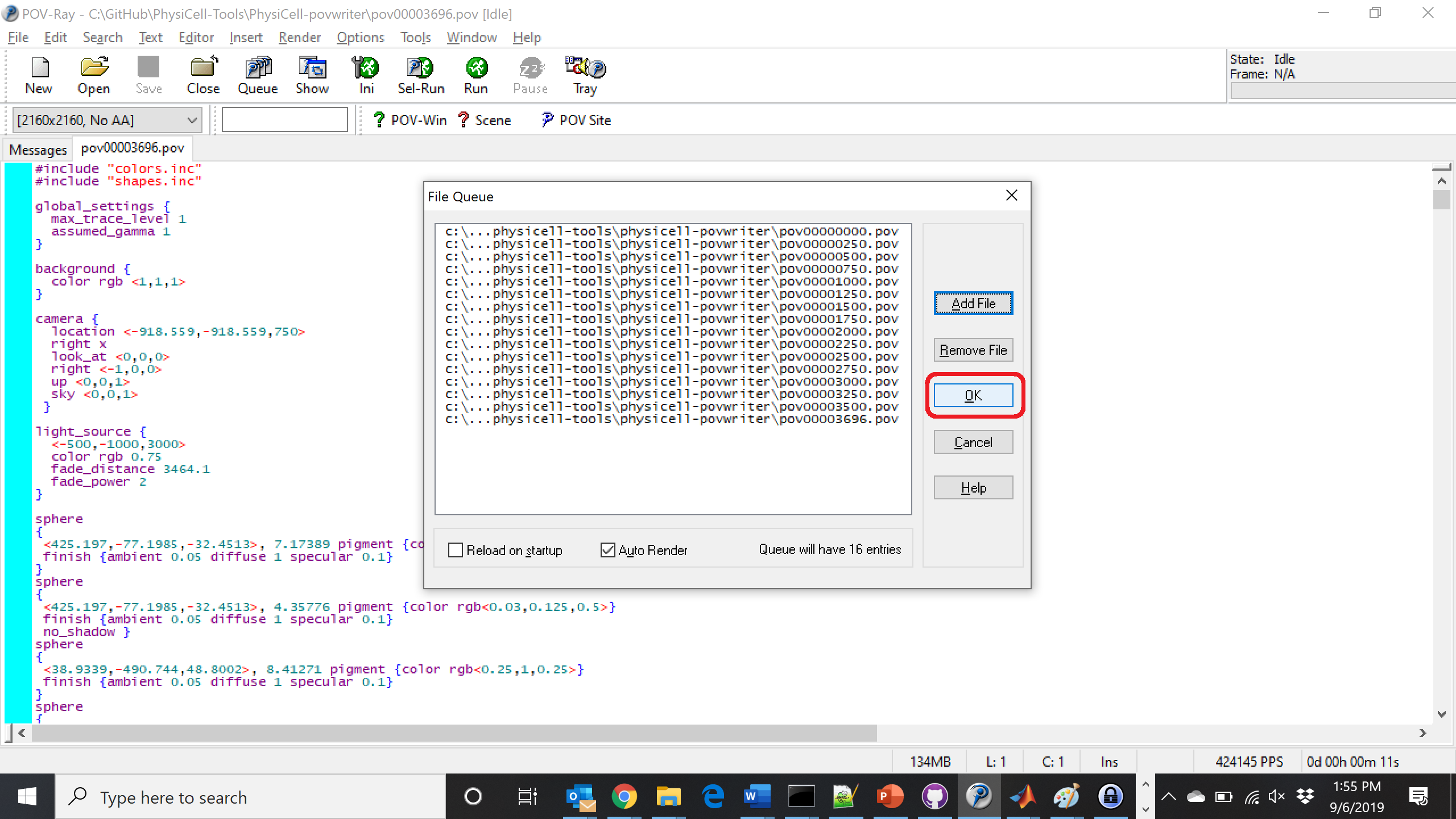
Now, go into POV-ray, and choose “queue.” Click “Add File” and select all 15 .pov files you just created:
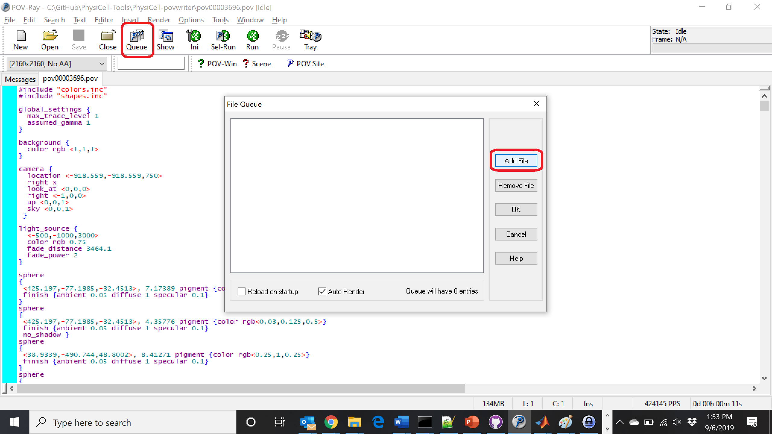
Hit “OK” to let it render all the povray files to create PNG files (pov00000000.png, … , pov00003500.png).
Using command-line options to process multiple times (option #2)
You can also give a list of indices. Here’s how we render time indices 250, 1000, and 2250:
physicell$ ./povwriter 250,1000,2250

povwriter version 1.0.0
================================================================================

Copyright (c) Paul Macklin 2019, on behalf of the PhysiCell project
OSI License: BSD-3-Clause (see LICENSE.txt)

Usage:
================================================================================
povwriter : run povwriter with config file ./config/settings.xml

povwriter FILENAME.xml : run povwriter with config file FILENAME.xml

povwriter x:y:z : run povwriter on data in FOLDER with indices from x
to y in incremenets of z

Example: ./povwriter 0:2:10 processes files:
./FOLDER/FILEBASE00000000_physicell_cells.mat
./FOLDER/FILEBASE00000002_physicell_cells.mat
...
./FOLDER/FILEBASE00000010_physicell_cells.mat
(See the config file to set FOLDER and FILEBASE)

povwriter x1,...,xn : run povwriter on data in FOLDER with indices x1,...,xn

Example: ./povwriter 1,3,17 processes files:
./FOLDER/FILEBASE00000001_physicell_cells.mat
./FOLDER/FILEBASE00000003_physicell_cells.mat
./FOLDER/FILEBASE00000017_physicell_cells.mat
(Note that there are no spaces.)
(See the config file to set FOLDER and FILEBASE)

Code updates at https://github.com/PhysiCell-Tools/PhysiCell-povwriter

Tutorial & documentation at http://MathCancer.org/blog/povwriter
================================================================================

Using config file ./config/povwriter-settings.xml ...
Using standard coloring function ...
Found 3 clipping planes ...
Found 2 cell color definitions ...
Processing file ./output/output00002250_cells_physicell.mat...
Matrix size: 32 x 37959
Creating file pov00002250.pov for output ...
Writing 37959 cells ...
Processing file ./output/output00001000_cells_physicell.mat...
Matrix size: 32 x 74057
Creating file pov00001000.pov for output ...
Processing file ./output/output00000250_cells_physicell.mat...
Matrix size: 32 x 75352
Writing 74057 cells ...
Creating file pov00000250.pov for output ...
Writing 75352 cells ...
done!

done!

done!

Done processing all 3 files!
This will create files pov00000250.pov, pov00001000.pov, and pov00002250.pov. Render them in POV-ray just as before.
Advanced options (at the source code level)
If you set use_standard_colors to false, povwriter uses the function my_pigment_and_finish_function (at the end of ./custom_modules/povwriter.cpp). Make sure that you set colors.cyto_pigment (RGB) and colors.nuclear_pigment (also RGB). The source file in povwriter has some hinting on how to write this. Note that the XML files saved by PhysiCell have a legend section that helps you do determine what is stored in each column of the matlab file.
Optional postprocessing
Image conversion / manipulation with ImageMagick
Suppose you want to convert the PNG files to JPEGs, and scale them down to 60% of original size. That’s very straightforward in ImageMagick:
physicell$ magick mogrify -format jpg -resize 60% pov*.png
Creating an animated GIF with ImageMagick
Suppose you want to create an animated GIF based on your images. I suggest first converting to JPG (see above) and then using ImageMagick again. Here, I’m adding a 20 ms delay between frames:
physicell$ magick convert -delay 20 *.jpg out.gif
Here’s the result:
Creating a compressed movie with Mencoder
Syntax coming later.
Closing thoughts and future work
In the future, we will probably allow more control over the clipping planes and a bit more debugging on how to handle planes that don’t pass through the origin. (First thoughts: we need to change how we use union and intersection commands in the POV-ray outputs.)
We should also look at adding some transparency for the cells. I’d prefer something like rgba (red-green-blue-alpha), but POV-ray uses filters and transmission, and we want to make sure to get it right.
Lastly, it would be nice to find a balance between the current very simple camera setup and better control.
Thanks for reading this PhysiCell Friday tutorial! Please do give PhysiCell at try (at http://PhysiCell.org) and read the method paper at PLoS Computational Biology.