Some quick math to calculate numerical convergence rates
I find myself needing to re-derive this often enough that it’s worth jotting down for current and future students. :-)
Introduction
A very common task in our field is to assess the convergence rate of a numerical algorithm: if I shrink \(\Delta t\) (or \(\Delta x\)), how quickly does my error shrink? And in fact, does my error shrink? Assuming you have a method to compute the error for a simulation (say, a simple test case where you know the exact solution), you want a fit an expression like this:
\[ \mathrm{Error}(\Delta t) = C \Delta t^n ,\] where \( C\) is a constant, and \( n \) is the order of convergence. Usually, if \( n \) isn’t at least 1, it’s bad.
So, suppose you are testing an algorithm, and you have the error \( E_1 \) for \( \Delta t_1 \) and \( E_2 \) for \( \Delta t_2 \). Then one way to go about this calculation is to try to cancel out \( C\):
\begin{eqnarray} \frac{ E_1}{E_2} = \frac{C \Delta t_1^n }{C \Delta t_2^n } = \left( \frac{ \Delta t_1 }{\Delta t_2} \right)^n & \Longrightarrow & n = \frac{ \log\left( E_1 / E_2 \right) }{ \log\left( \Delta t_1 / \Delta t_2 \right) } \end{eqnarray}
Another way to look at this problem is to rewrite the error equation in log-log space:
\begin{eqnarray} E = C \Delta t^N & \Longrightarrow & \log{E} = \log{C} + n \log{ \Delta t} \end{eqnarray}
so \(n\) is the slope of the equation in log space. If you only have two points, then,
\[ n = \frac{ \log{E_1} – \log{E_2} }{ \log{\Delta t_1} – \log{\Delta t_1} } = \frac{ \log\left( E_1 / E_2 \right) }{ \log\left( \Delta t_1 / \Delta t_2 \right) }, \] and so we end up with the exact same convergence rate as before.
However, if you have calculated the error \( E_i \) for a whole bunch of values \( \Delta t_i \), then you can extend this idea to get a better sense of the overall convergence rate for all your values of \( \Delta t \), rather than just two values. Just find the linear least squares fit to the points \( \left\{ ( \log\Delta t_i, \log E_i ) \right\} \). If there are just two points, it’s the same as above. If there are many, it’s a better representation of overall convergence.
Trying it out
Let’s demonstrate this on a simple test problem:
\[ \frac{du}{dt} = -10 u, \hspace{.5in} u(0) = 1.\]
We’ll simulate using (1st-order) forward Euler and (2nd-order) Adams-Bashforth:
dt_vals = [.2 .1 .05 .01 .001 .0001];

min_t = 0;
max_t = 1;

lambda = 10;
initial = 1;

errors_forward_euler = [];
errors_adams_bashforth = [];

for j=1:length( dt_vals )
    dt = dt_vals(j);
    T = min_t:dt:max_t;

    % allocate memory

    solution_forward_euler = zeros(1,length(T));
    solution_forward_euler(1) = initial;
    solution_adams_bashforth = solution_forward_euler;

    % exact solution

    solution_exact = initial * exp( -lambda * T );

    % forward euler

    for i=2:length(T)
        solution_forward_euler(i) = solution_forward_euler(i-1)...
            - dt*lambda*solution_forward_euler(i-1);
    end

    % adams-bashforth -- use high-res Euler to jump-start

    dt_fine = dt * 0.1;
    t = min_t + dt_fine;
    temp = initial ;
    for i=1:10
        temp = temp - dt_fine*lambda*temp;
    end
    solution_adams_bashforth(2) = temp;

    for i=3:length(T)
        solution_adams_bashforth(i) = solution_adams_bashforth(i-1)...
            - 0.5*dt*lambda*( 3*solution_adams_bashforth(i-1)...
            - solution_adams_bashforth(i-2 ) );
    end

%     Uncomments if you want to see plots.
%     figure(1)
%     clf;
%     plot( T, solution_exact, 'r*' , T , solution_forward_euler,...
%         'b-o', T , solution_adams_bashforth , 'k-s'  );
%     pause ;

    errors_forward_euler(j) = ...
        max(abs( solution_exact - solution_forward_euler ) );
    errors_adams_bashforth(j) = ...
        max(abs( solution_exact - solution_adams_bashforth ) );

end
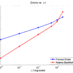
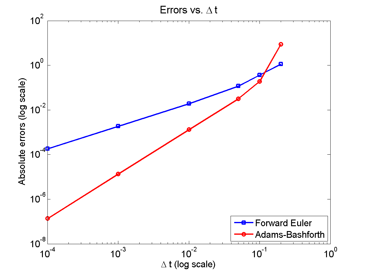
Here is a plot of the errors:
figure(2)
loglog( dt_vals, errors_forward_euler, 'b-s' ,...
    dt_vals, errors_adams_bashforth, 'r-o' ,...
    'linewidth', 2 );
legend( 'Forward Euler', 'Adams-Bashforth' , 4 );
xlabel( '\Delta t (log scale)' , 'fontsize', 14 );
ylabel( 'Absolute errors (log scale)', 'fontsize', 14 );
title( 'Errors vs. \Delta t', 'fontsize' , 16 );
set( gca, 'fontsize' , 14 );
Note that calculating the convergence rate based on the first two errors, and first and last errors, is not terribly
representative, compared with using all the errors:
% Convergence rate based on the first two errors
polyfit( log(dt_vals(1:2)) , log(errors_forward_euler(1:2)) , 1 )
polyfit( log(dt_vals(1:2)) , log(errors_adams_bashforth(1:2)) , 1 )

% Convergence rate based on the first and last errors
m = length(dt_vals);
polyfit( log( [dt_vals(1),dt_vals(m)] ) ,...
    log( [errors_forward_euler(1),errors_forward_euler(m)]) , 1 )
polyfit( log( [dt_vals(1),dt_vals(m)] ) ,...
    log( [errors_adams_bashforth(1),errors_adams_bashforth(m)]) , 1 )

% Convergence rate based on all the errors
polyfit( log(dt_vals) , log(errors_forward_euler) , 1 )
polyfit( log(dt_vals) , log(errors_adams_bashforth) , 1 )

% Convergence rate based on all the errors but the outlier
polyfit( log(dt_vals(2:m)) , log(errors_forward_euler(2:m)) , 1 )
polyfit( log(dt_vals(2:m)) , log(errors_adams_bashforth(2:m)) , 1 )
Using the first two errors gives a convergence rate over 5 for Adams-Bashforth, and around 1.6 for forward Euler. Using first and last is better, but still over-estimates the convergence rates (1.15 and 2.37, FE and AB, respectively). Linear least squares is closer to reality: 1.12 for FE, 2.21 for AB. And lastly, linear least squares but excluding the outliers, we get 1.08 for forward Euler, and 2.03 for Adams-Bashforth. (As expected!)
Which convergence rates are “right”?
So, which values do you report as your convergence rates? Ideally, use all the errors to avoid bias and/or cherry-picking. It’s the most honest and straightforward way to present the work. However, you may have a good rationale to exclude the clear outliers in this case. But then again, if you have calculated the errors for enough values of \(\Delta t\), there’s no need to do this at all. There’s little value in (or basis for) reporting the convergence rate to three significant digits. I’d instead report these as approximately first-order convergence (forward Euler) and approximately second-order convergence (Adams-Bashforth); we get this result with either linear least squares fit, and using all your data points puts you on more solid ground.
Return to News • Return to MathCancer • Follow @MathCancer