Running the PhysiCell sample projects
Introduction
In PhysiCell 1.2.1 and later, we include four sample projects on cancer heterogeneity, bioengineered multicellular systems, and cancer immunology. This post will walk you through the steps to build and run the examples.
If you are new to PhysiCell, you should first make sure you’re ready to run it. (Please note that this applies in particular for OSX users, as Xcode’s g++ is not compatible out-of-the-box.) Here are tutorials on getting ready to Run PhysiCell:
- Setting up a 64-bit gcc environment in Windows.
- Setting up gcc / OpenMP on OSX (MacPorts edition)
- Setting up gcc / OpenMP on OSX (Homebrew edition)
Note: This is the preferred method for Mac OSX. - Getting started with a PhysiCell Virtual Appliance (for virtual machines like VirtualBox)
Note: The “native” setups above are preferred, but the Virtual Appliance is a great “plan B” if you run into trouble
Please note that we expect to expand this tutorial.
Building, running, and viewing the sample projects
All of these projects will create data of the following forms:
- Scalable vector graphics (SVG) cross-section plots through z = 0.0 μm at each output time. Filenames will look like snapshot00000000.svg.
- Matlab (Level 4) .mat files to store raw BioFVM data. Filenames will look like output00000000_microenvironment0.mat (for the chemical substrates) and output00000000_cells.mat (for basic agent data).
- Matlab .mat files to store additional PhysiCell agent data. Filenames will look like output00000000_cells_physicell.mat.
- MultiCellDS .xml files that give further metadata and structure for the .mat files. Filenames will look like output00000000.xml.
You can read the combined data in the XML and MAT files with the read_MultiCellDS_xml function, stored in the matlab directory of every PhysiCell download. (Copy the read_MultiCellDS_xml.m and set_MultiCelLDS_constants.m files to the same directory as your data for the greatest simplicity.)
(If you are using Mac OSX and PhysiCell version > 1.2.1, remember to set the PHYSICELL_CPP environment variable to be an OpenMP-capable compiler – rf. Homebrew setup.)
Biorobots (2D)
Type the following from a terminal window in your root PhysiCell directory:
make biorobots-sample
make
./biorobots
make reset # optional -- gets a clean slate to try other samples
Because this is a 2-D example, the SVG snapshot files will provide the simplest method of visualizing these outputs. You can use utilities like ImageMagick to convert them into other formats for publications, such as PNG or EPS.
Anti-cancer biorobots (2D)
make cancer-biorobots-sample
make
./cancer_biorobots
make reset # optional -- gets a clean slate to try other samples
Cancer heterogeneity (2D)
make heterogeneity-sample
make project
./heterogeneity
make reset # optional -- gets a clean slate to try other samples
Cancer immunology (3D)
make cancer-immune-sample
make
./cancer_immune_3D
make reset # optional -- gets a clean slate to try other samples
A small computational thought experiment
In Macklin (2017), I briefly touched on a simple computational thought experiment that shows that for a group of homogeneous cells, you can observe substantial heterogeneity in cell behavior. This “thought experiment” is part of a broader preview and discussion of a fantastic paper by Linus Schumacher, Ruth Baker, and Philip Maini published in Cell Systems, where they showed that a migrating collective homogeneous cells can show heterogeneous behavior when quantitated with new migration metrics. I highly encourage you to check out their work!
In this blog post, we work through my simple thought experiment in a little more detail.
Note: If you want to reference this blog post, please cite the Cell Systems preview article:
P. Macklin, When seeing isn’t believing: How math can guide our interpretation of measurements and experiments. Cell Sys., 2017 (in press). DOI: 10.1016/j.cells.2017.08.005
The thought experiment
Consider a simple (and widespread) model of a population of cycling cells: each virtual cell (with index i) has a single “oncogene” \( r_i \) that sets the rate of progression through the cycle. Between now (t) and a small time from now ( \(t+\Delta t\)), the virtual cell has a probability \(r_i \Delta t\) of dividing into two daughter cells. At the population scale, the overall population growth model that emerges from this simple single-cell model is:
\[\frac{dN}{dt} = \langle r\rangle N, \]
where \( \langle r \rangle \) the mean division rate over the cell population, and N is the number of cells. See the discussion in the supplementary information for Macklin et al. (2012).
Now, suppose (as our thought experiment) that we could track individual cells in the population and track how long it takes them to divide. (We’ll call this the division time.) What would the distribution of cell division times look like, and how would it vary with the distribution of the single-cell rates \(r_i\)?
Mathematical method
In the Matlab script below, we implement this cell cycle model as just about every discrete model does. Here’s the pseudocode:
t = 0;
while( t < t_max )
    for i=1:Cells.size()
        u = random_number();
        if( u < Cells[i].birth_rate * dt )
            Cells[i].division_time = Cells[i].age;
            Cells[i].divide();
        end
    end
    t = t+dt;
end
That is, until we’ve reached the final simulation time, loop through all the cells and decide if they should divide: For each cell, choose a random number between 0 and 1, and if it’s smaller than the cell’s division probability (\(r_i \Delta t\)), then divide the cell and write down the division time.
As an important note, we have to track the same cells until they all divide, rather than merely record which cells have divided up to the end of the simulation. Otherwise, we end up with an observational bias that throws off our recording. See more below.
The sample code
You can download the Matlab code for this example at:
http://MathCancer.org/files/matlab/thought_experiment_matlab(Macklin_Cell_Systems_2017).zip
Extract all the files, and run “thought_experiment” in Matlab (or Octave, if you don’t have a Matlab license or prefer an open source platform) for the main result.
All these Matlab files are available as open source, under the GPL license (version 3 or later).
Results and discussion
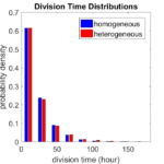
First, let’s see what happens if all the cells are identical, with \(r = 0.05 \textrm{ hr}^{-1}\). We run the script, and track the time for each of 10,000 cells to divide. As expected by theory (Macklin et al., 2012) (but perhaps still a surprise if you haven’t looked), we get an exponential distribution of division times, with mean time \(1/\langle r \rangle\):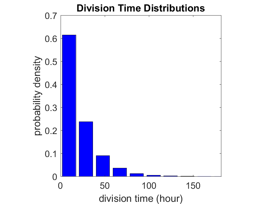
So even in this simple model, a homogeneous population of cells can show heterogeneity in their behavior. Here’s the interesting thing: let’s now give each cell its own division parameter \(r_i\) from a normal distribution with mean \(0.05 \textrm{ hr}^{-1}\) and a relative standard deviation of 25%: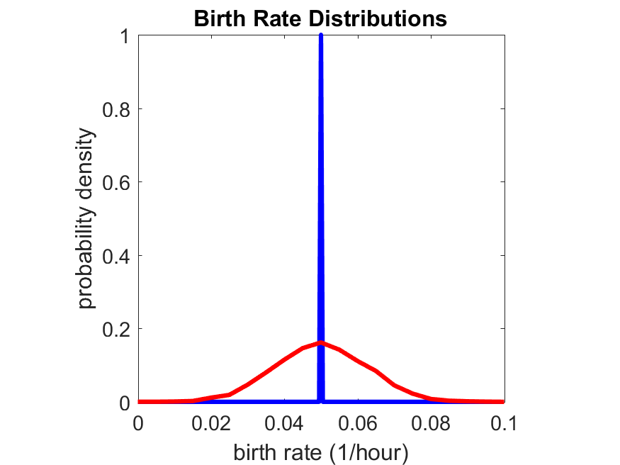
If we repeat the experiment, we get the same distribution of cell division times!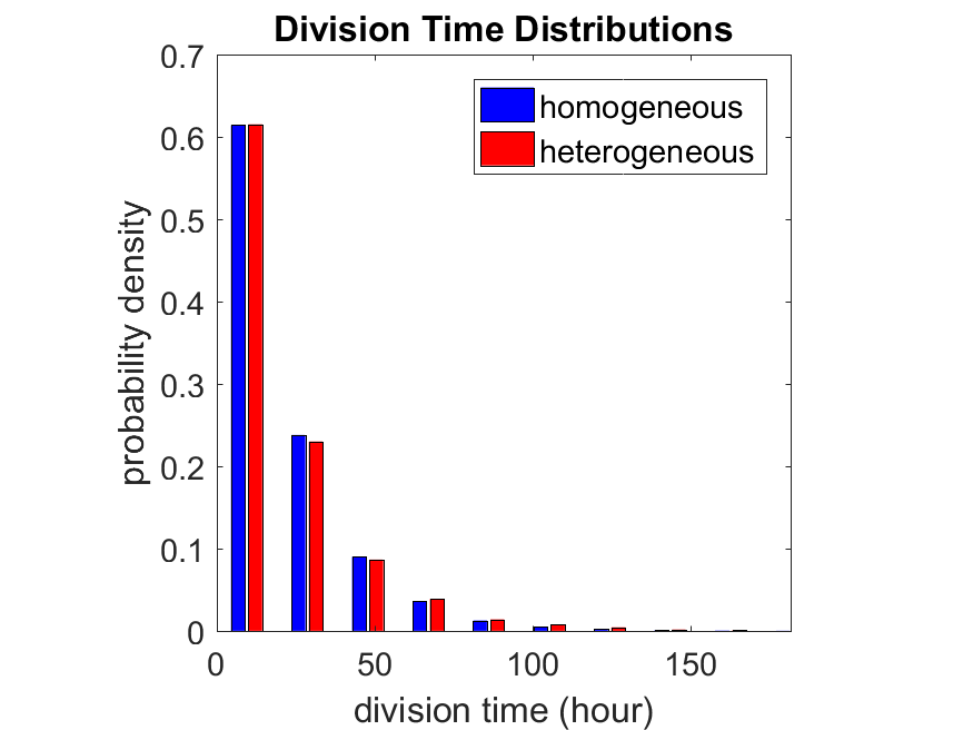
So in this case, based solely on observations of the phenotypic heterogeneity (the division times), it is impossible to distinguish a “genetically” homogeneous cell population (one with identical parameters) from a truly heterogeneous population. We would require other metrics, like tracking changes in the mean division time as cells with a higher \(r_i\) out-compete the cells with lower \(r_i\).
Lastly, I want to point out that caution is required when designing these metrics and single-cell tracking. If instead we had tracked all cells throughout the simulated experiment, including new daughter cells, and then recorded the first 10,000 cell division events, we would get a very different distribution of cell division times: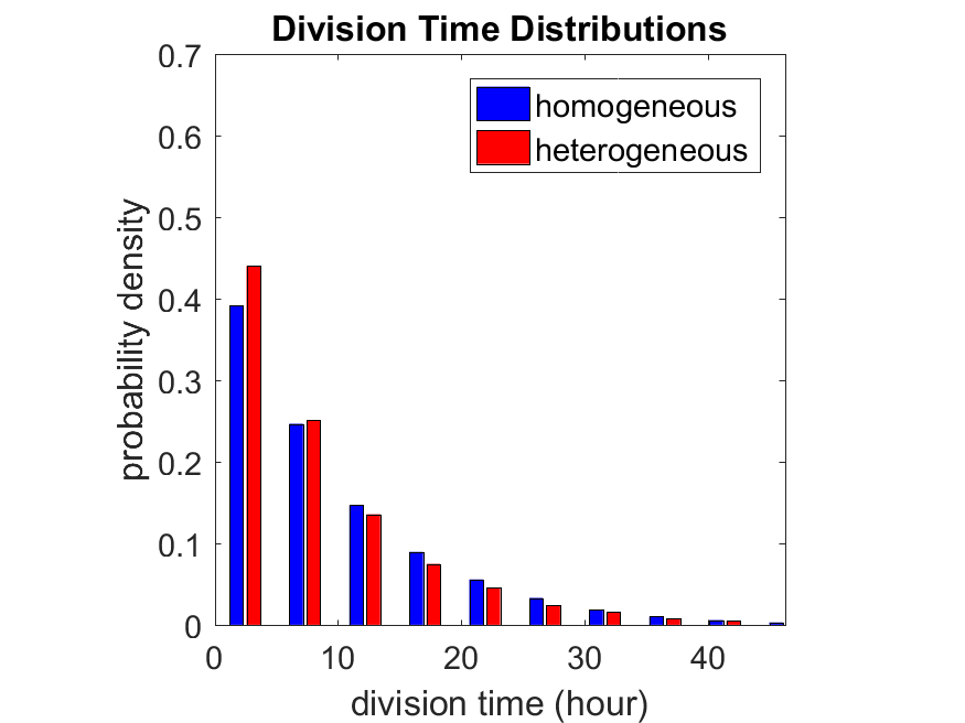
By only recording the division times for the cells that have divided, and not those that haven’t, we bias our observations towards cells with shorter division times. Indeed, the mean division time for this simulated experiment is far lower than we would expect by theory. You can try this one by running “bad_thought_experiment”.
Further reading
This post is an expansion of our recent preview in Cell Systems in Macklin (2017):
P. Macklin, When seeing isn’t believing: How math can guide our interpretation of measurements and experiments. Cell Sys., 2017 (in press). DOI: 10.1016/j.cells.2017.08.005
And the original work on apparent heterogeneity in collective cell migration is by Schumacher et al. (2017):
L. Schumacher et al., Semblance of Heterogeneity in Collective Cell Migration. Cell Sys., 2017 (in press). DOI: 10.1016/j.cels.2017.06.006
You can read some more on relating exponential distributions and Poisson processes to common discrete mathematical models of cell populations in Macklin et al. (2012):
P. Macklin, et al., Patient-calibrated agent-based modelling of ductal carcinoma in situ (DCIS): From microscopic measurements to macroscopic predictions of clinical progression. J. Theor. Biol. 301:122-40, 2012. DOI: 10.1016/j.jtbi.2012.02.002.
Lastly, I’d be delighted if you took a look at the open source software we have been developing for 3-D simulations of multicellular systems biology:
http://OpenSource.MathCancer.org
And you can always keep up-to-date by following us on Twitter: @MathCancer.
Getting started with a PhysiCell Virtual Appliance
Note: This is part of a series of “how-to” blog posts to help new users and developers of BioFVM and PhysiCell. This guide is for for users in OSX, Linux, or Windows using the VirtualBox virtualization software to run a PhysiCell virtual appliance.
These instructions should get you up and running without needed to install a compiler, makefile capabilities, or any other software (beyond the virtual machine and the PhysiCell virtual appliance). We note that using the PhysiCell source with your own compiler is still the preferred / ideal way to get started, but the virtual appliance option is a fast way to start even if you’re having troubles setting up your development environment.
What’s a Virtual Machine? What’s a Virtual Appliance?
A virtual machine is a full simulated computer (with its own disk space, operating system, etc.) running on another. They are designed to let a user test on a completely different environment, without affecting the host (main) environment. They also allow a very robust way of taking and reproducing the state of a full working environment.
A virtual appliance is just this: a full image of an installed system (and often its saved state) on a virtual machine, which can easily be installed on a new virtual machine. In this tutorial, you will download our PhysiCell virtual appliance and use its pre-configured compiler and other tools.
What you’ll need:
- VirtualBox: This is a free, cross-platform program to run virtual machines on OSX, Linux, Windows, and other platforms. It is a safe and easy way to install one full operating (a client system) on your main operating system (the host system). For us, this means that we can distribute a fully working Linux environment with a working copy of all the tools you need to compile and run PhysiCell. As of August 1, 2017, this will download Version 5.1.26.
- Download here: https://www.virtualbox.org/wiki/Downloads
- PhysiCell Virtual Appliance: This is a single-file distribution of a virtual machine running Alpine Linux, including all key tools needed to compile and run PhysiCell. As of July 31, 2017, this will download PhysiCell 1.2.2 with g++ 6.3.0.
- Download here: https://sourceforge.net/projects/physicell/files/PhysiCell/
- (Browse to a version of PhysiCell, and download the file that ends in “.ova”.)
- Version 1.2.0: http://bit.ly/2vY51P1 [sf.net]
- Download here: https://sourceforge.net/projects/physicell/files/PhysiCell/
- A computer with hardware support for virtualization: Your CPU needs to have hardware support for virtualization (almost all of them do now), and it has to be enabled in your BIOS. Consult your computer maker on how to turn this on if you get error messages later.
Main steps:
1) Install VirtualBox.
Double-click / open the VirtualBox download. Go ahead and accept all the default choices. If asked, go ahead and download/install the extensions pack.
2) Import the PhysiCell Virtual Appliance
Go the “File” menu and choose “Import Virtual Appliance”. Browse to find the .ova file you just downloaded.
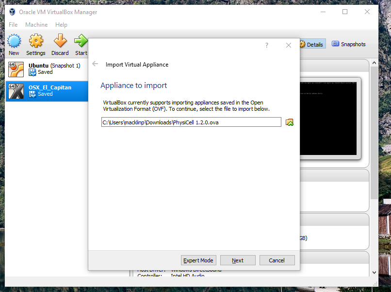
Click on “Next,” and import with all the default options. That’s it!
3) [Optional] Change settings
You most likely won’t need this step, but you can increase/decrease the amount of RAM used for the virtual machine if you select the PhysiCell VM, click the Settings button (orange gear), and choose “System”: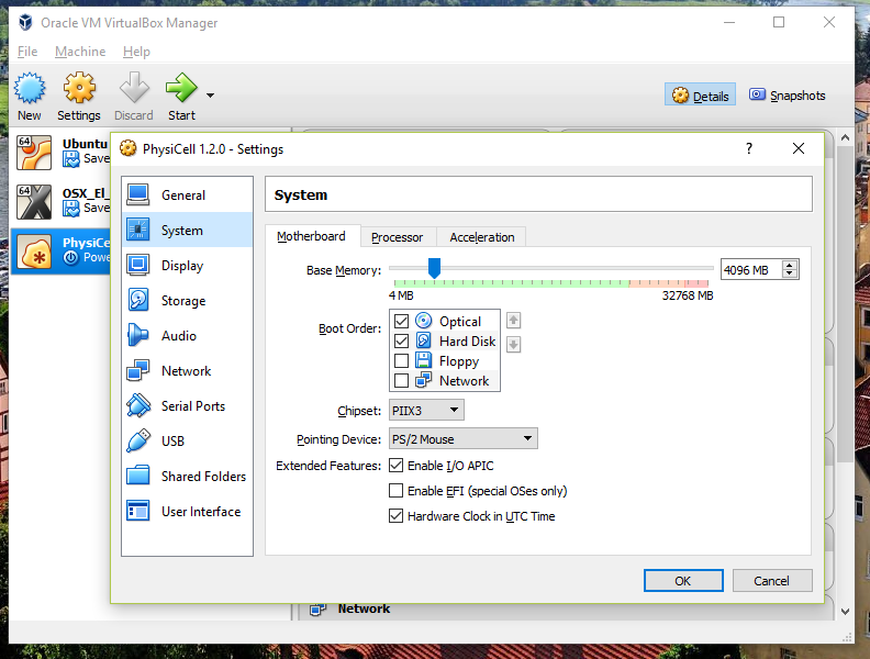 We set the Virtual Machine to have 4 GB of RAM. If you have a machine with lots of RAM (16 GB or more), you may want to set this to 8 GB.
Also, you can choose how many virtual CPUs to give to your VM: 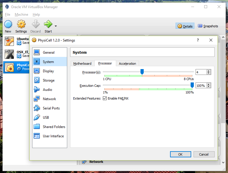
We selected 4 when we set up the Virtual Appliance, but you should match the number of physical processor cores on your machine. In my case, I have a quad core processor with hyperthreading. This means 4 real cores, 8 virtual cores, so I select 4 here.
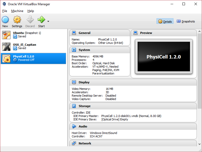
4) Start the Virtual Machine and log in
Select the PhysiCell machine, and click the green “start” button. After the virtual machine boots (with the good old LILO boot manager that I’ve missed), you should see this:
Click the "More ..." button, and log in with username: physicell, password: physicell
5) Test the compiler and run your first simulation
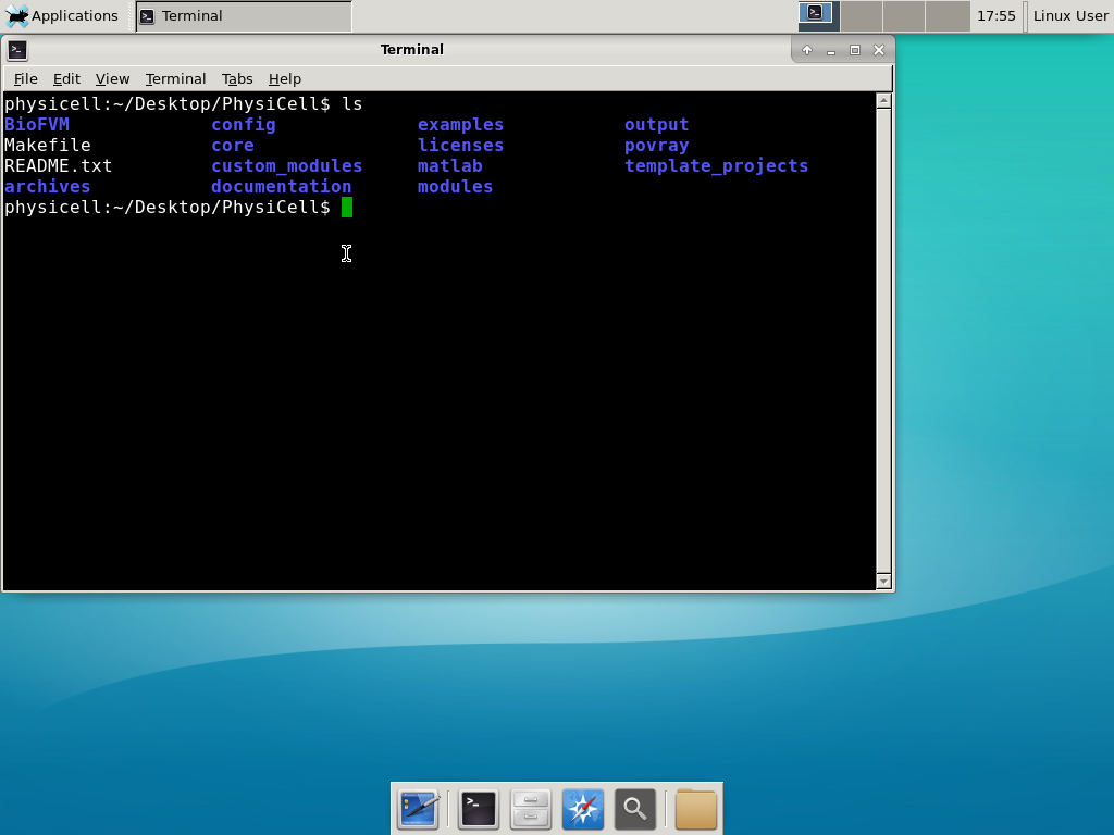
Notice that PhysiCell is already there on the desktop in the PhysiCell folder. Right-click, and choose “open terminal here.” You’ll already be in the main PhysiCell root directory. 
Now, let’s compile your first project! Type “make template2D && make” 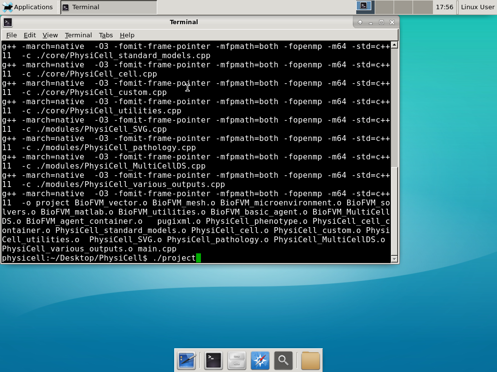 And run your project! Type “./project” and let it go!
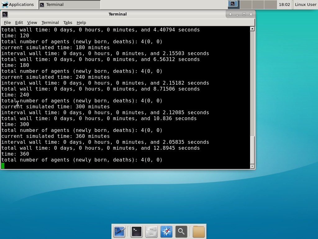 Go ahead and run either the first few days of the simulation (until about 7200 minutes), then hit <control>-C to cancel out. Or run the whole simulation–that’s fine, too.
6) Look at the results
We bundled a few tools to easily look at results. First, ristretto is a very fast image viewer. Let’s view the SVG files: 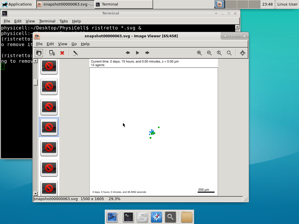 As a nice tip, you can press the left and right arrows to advance through the SVG images, or hold the right arrow down to advance through quickly.
Now, let’s use ImageMagick to convert the SVG files into JPG file: call “magick mogrify -format jpg snap*.svg”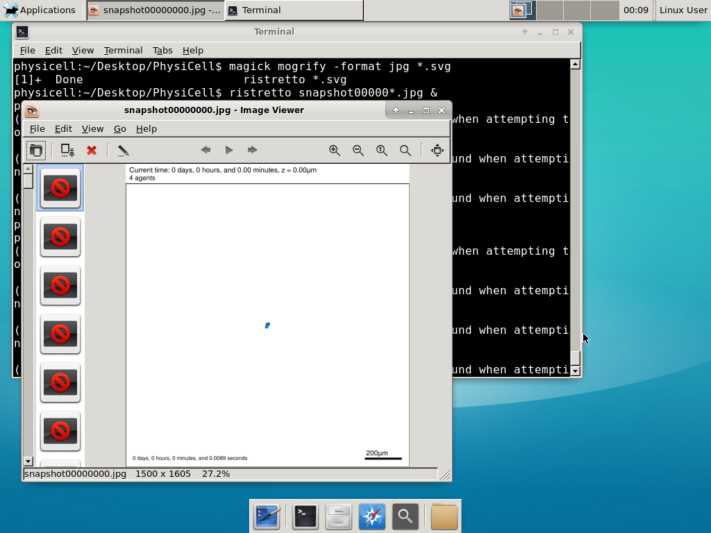
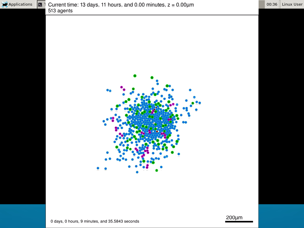
Next, let’s turn those images into a movie. I generally create moves that are 24 frames pers se, so that 1 second of the movie is 1 hour of simulations time. We’ll use mencoder, with options below given to help get a good quality vs. size tradeoff: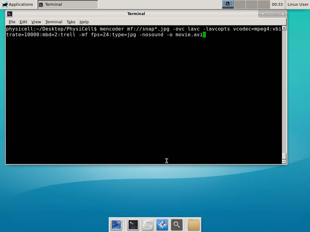
When you’re done, view the movie with mplayer. The options below scale the window to fit within the virtual monitor:
If you want to loop the movie, add “-loop 999” to your command.
7) Get familiar with other tools
Use nano (useage: nano <filename>) to quickly change files at the command line. Hit <control>-O to save your results. Hit <control>-X to exit. <control>-W will search within the file.
Use nedit (useage: nedit <filename> &) to open up one more text files in a graphical editor. This is a good way to edit multiple files at once.
Sometimes, you need to run commands at elevated (admin or root) privileges. Use sudo. Here’s an example, searching the Alpine Linux package manager apk for clang:
physicell:~$ sudo apk search gcc
[sudo] password for physicell:
physicell:~$ sudo apk search clang
clang-analyzer-4.0.0-r0
clang-libs-4.0.0-r0
clang-dev-4.0.0-r0
clang-static-4.0.0-r0
emscripten-fastcomp-1.37.10-r0
clang-doc-4.0.0-r0
clang-4.0.0-r0
physicell:~/Desktop/PhysiCell$
If you want to install clang/llvm (as an alternative compiler):
physicell:~$ sudo apk add gcc
[sudo] password for physicell:
physicell:~$ sudo apk search clang
clang-analyzer-4.0.0-r0
clang-libs-4.0.0-r0
clang-dev-4.0.0-r0
clang-static-4.0.0-r0
emscripten-fastcomp-1.37.10-r0
clang-doc-4.0.0-r0
clang-4.0.0-r0
physicell:~/Desktop/PhysiCell$
Notice that it asks for a password: use the password for root (which is physicell).
8) [Optional] Configure a shared folder
Coming soon.
Why both with zipped source, then?
Given that we can get a whole development environment by just downloading and importing a virtual appliance, why
bother with all the setup of a native development environment, like this tutorial (Windows) or this tutorial (Mac)?
One word: performance. In my testing, I still have not found the performance running inside a
virtual machine to match compiling and running directly on your system. So, the Virtual Appliance is a great
option to get up and running quickly while trying things out, but I still recommend setting up natively with
one of the tutorials I linked in the preceding paragraphs.
What’s next?
In the coming weeks, we’ll post further tutorials on using PhysiCell. In the meantime, have a look at the
PhysiCell project website, and these links as well:
- BioFVM on MathCancer.org: http://BioFVM.MathCancer.org
- BioFVM on SourceForge: http://BioFVM.sf.net
- BioFVM Method Paper in BioInformatics: http://dx.doi.org/10.1093/bioinformatics/btv730
- PhysiCell on MathCancer.org: http://PhysiCell.MathCancer.org
- PhysiCell on Sourceforge: http://PhysiCell.sf.net
- PhysiCell Method Paper (preprint): https://doi.org/10.1101/088773
- PhysiCell tutorials: [click here]
MathCancer C++ Style and Practices Guide
As PhysiCell, BioFVM, and other open source projects start to gain new users and contributors, it’s time to lay out a coding style. We have three goals here:
- Consistency: It’s easier to understand and contribute to the code if it’s written in a consistent way.
- Readability: We want the code to be as readable as possible.
- Reducing errors: We want to avoid coding styles that are more prone to errors. (e.g., code that can be broken by introducing whitespace).
So, here is the guide (revised June 2017). I expect to revise this guide from time to time.
Place braces on separate lines in functions and classes.
I find it much easier to read a class if the braces are on separate lines, with good use of whitespace. Remember: whitespace costs almost nothing, but reading and understanding (and time!) are expensive.
DON’T
class Cell{
public:
 double some_variable;
 bool some_extra_variable;

 Cell(); };

class Phenotype{
public:
 double some_variable;
 bool some_extra_variable;

 Phenotype();
};
DO:
class Cell
{
 public:
     double some_variable;
     bool some_extra_variable;

     Cell();
};

class Phenotype
{
 public:
     double some_variable;
     bool some_extra_variable;

     Phenotype();
};
Enclose all logic in braces, even when optional.
In C/C++, you can omit the curly braces in some cases. For example, this is legal
if( distance > 1.5*cell_radius )
     interaction = false;
force = 0.0; // is this part of the logic, or a separate statement?
error = false;
However, this code is ambiguous to interpret. Moreover, small changes to whitespace–or small additions to the logic–could mess things up here. Use braces to make the logic crystal clear:
DON’T
if( distance > 1.5*cell_radius )
     interaction = false;
force = 0.0; // is this part of the logic, or a separate statement?
error = false;

if( condition1 == true )
  do_something1 = true;
elseif( condition2 == true )
  do_something2 = true;
else
  do_something3 = true;
DO
if( distance > 1.5*cell_radius )
{
     interaction = false;
     force = 0.0;
}
error = false;

if( condition1 == true )
{ do_something1 = true; }
elseif( condition2 == true )
{ do_something2 = true; }
else
{ do_something3 = true; }
Put braces on separate lines in logic, except for single-line logic.
This style rule relates to the previous point, to improve readability.
DON’T
if( distance > 1.5*cell_radius ){
     interaction = false;
     force = 0.0; }

if( condition1 == true ){ do_something1 = true; }
elseif( condition2 == true ){
  do_something2 = true; }
else
{ do_something3 = true; error = true; }
DO
if( distance > 1.5*cell_radius )
{
     interaction = false;
     force = 0.0;
}

if( condition1 == true )
{ do_something1 = true; } // this is fine
elseif( condition2 == true )
{
     do_something2 = true; // this is better
}
else
{
     do_something3 = true;
     error = true;
}
See how much easier that code is to read? The logical structure is crystal clear, and adding more to the logic is simple.
End all functions with a return, even if void.
For clarity, definitively state that a function is done by using return.
DON’T
void my_function( Cell& cell )
{
     cell.phenotype.volume.total *= 2.0;
     cell.phenotype.death.rates[0] = 0.02;
     // Are we done, or did we forget something?
     // is somebody still working here?
}
DO
void my_function( Cell& cell )
{
     cell.phenotype.volume.total *= 2.0;
     cell.phenotype.death.rates[0] = 0.02;
     return;
}
Use tabs to indent the contents of a class or function.
This is to make the code easier to read. (Unfortunately PHP/HTML makes me use five spaces here instead of tabs.)
DON’T
class Secretion
{
 public:
std::vector<double> secretion_rates;
std::vector<double> uptake_rates;
std::vector<double> saturation_densities;
};

void my_function( Cell& cell )
{
cell.phenotype.volume.total *= 2.0;
cell.phenotype.death.rates[0] = 0.02;
return;
}
DO
class Secretion
{
 public:
     std::vector<double> secretion_rates;
     std::vector<double> uptake_rates;
     std::vector<double> saturation_densities;
};

void my_function( Cell& cell )
{
     cell.phenotype.volume.total *= 2.0;
     cell.phenotype.death.rates[0] = 0.02;
     return;
}
Use a single space to indent public and other keywords in a class.
This gets us some nice formatting in classes, without needing two tabs everywhere.
DON’T
class Secretion
{
public:
std::vector<double> secretion_rates;
std::vector<double> uptake_rates;
std::vector<double> saturation_densities;
}; // not enough whitespace

class Errors
{
     private:
          std::string none_of_your_business
     public:
          std::string error_message;
          int error_code;
}; // too much whitespace!
DO
class Secretion
{
 private:
 public:
     std::vector<double> secretion_rates;
     std::vector<double> uptake_rates;
     std::vector<double> saturation_densities;
};

class Errors
{
 private:
     std::string none_of_your_business
 public:
     std::string error_message;
     int error_code;
};
Avoid arcane operators, when clear logic statements will do.
It can be difficult to decipher code with statements like this:
phenotype.volume.fluid=phenotype.volume.fluid<0?0:phenotype.volume.fluid;
Moreover, C and C++ can treat precedence of ternary operators very differently, so subtle bugs can creep in when using the “fancier” compact operators. Variations in how these operators work across languages are an additional source of error for programmers switching between languages in their daily scientific workflows. Wherever possible (and unless there is a significant performance reason to do so), use clear logical structures that are easy to read even if you only dabble in C/C++. Compiler-time optimizations will most likely eliminate any performance gains from these goofy operators.
DON’T
// if the fluid volume is negative, set it to zero
phenotype.volume.fluid=phenotype.volume.fluid<0.0?0.0:pCell->phenotype.volume.fluid;
DO
if( phenotype.volume.fluid < 0.0 )
{
     phenotype.volume.fluid = 0.0;
}
Here’s the funny thing: the second logic is much clearer, and it took fewer characters, even with extra whitespace for readability!
Pass by reference where possible.
Passing by reference is a great way to boost performance: we can avoid (1) allocating new temporary memory, (2) copying data into the temporary memory, (3) passing the temporary data to the function, and (4) deallocating the temporary memory once finished.
DON’T
double some_function( Cell cell )
{
     return = cell.phenotype.volume.total + 3.0;
}
// This copies cell and all its member data!
DO
double some_function( Cell& cell )
{
     return = cell.phenotype.volume.total + 3.0;
}
// This just accesses the original cell data without recopying it.
Where possible, pass by reference instead of by pointer.
There is no performance advantage to passing by pointers over passing by reference, but the code is simpler / clearer when you can pass by reference. It makes code easier to write and understand if you can do so. (If nothing else, you save yourself character of typing each time you can replace “->” by “.”!)
DON’T
double some_function( Cell* pCell )
{
     return = pCell->phenotype.volume.total + 3.0;
}
// Writing and debugging this code can be error-prone.
DO
double some_function( Cell& cell )
{
     return = cell.phenotype.volume.total + 3.0;
}
// This is much easier to write.
Be careful with static variables. Be thread safe!
PhysiCell relies heavily on parallelization by OpenMP, and so you should write functions under the assumption that they may be executed many times simultaneously. One easy source of errors is in static variables:
DON’T
double some_function( Cell& cell )
{
     static double four_pi = 12.566370614359172;
     static double output;
     output = cell.phenotype.geometry.radius;
     output *= output;
     output *= four_pi;
     return output;
}
// If two instances of some_function are running, they will both modify
// the *same copy* of output
DO
double some_function( Cell& cell )
{
     static double four_pi = 12.566370614359172;
     double output;
     output = cell.phenotype.geometry.radius;
     output *= output;
     output *= four_pi;
     return output;
}
// If two instances of some_function are running, they will both modify
// the their own copy of output, but still use the more efficient, once-
// allocated copy of four_pi. This one is safe for OpenMP.
Use std:: instead of “using namespace std”
PhysiCell uses the BioFVM and PhysiCell namespaces to avoid potential collision with other codes. Other codes using PhysiCell may use functions that collide with the standard namespace. So, we formally use std:: whenever using functions in the standard namespace.
DON’T
using namespace std;

cout << "Hi, Mom, I learned to code today!" << endl;
string my_string = "Cheetos are good, but Doritos are better.";
cout << my_string << endl;

vector<double> my_vector;
vector.resize( 3, 0.0 );
DO
std::cout << "Hi, Mom, I learned to code today!" << std::endl;
std::string my_string = "Cheetos are good, but Doritos are better.";
std::cout << my_string << std::endl;

std::vector<double> my_vector;
my_vector.resize( 3, 0.0 );
Camelcase is ugly. Use underscores.
This is purely an aesthetic distinction, but CamelCaseCodeIsUglyAndDoYouUseDNAorDna?
DON’T
double MyVariable1;
bool ProteinsInExosomes;
int RNAtranscriptionCount;

void MyFunctionDoesSomething( Cell& ImmuneCell );
DO
double my_variable1;
bool proteins_in_exosomes;
int RNA_transcription_count;

void my_function_does_something( Cell& immune_cell );
Use capital letters to declare a class. Use lowercase for instances.
To help in readability and consistency, declare classes with capital letters (but no camelcase), and use lowercase for instances of those classes.
DON’T
class phenotype;

class cell
{
 public:
     std::vector<double> position;
     phenotype Phenotype;
};

class ImmuneCell : public cell
{
 public:
     std::vector<double> surface_receptors;
};

void do_something( cell& MyCell , ImmuneCell& immuneCell );

cell Cell;
ImmuneCell MyImmune_cell;

do_something( Cell, MyImmune_cell );
DO
class Phenotype;

class Cell
{
 public:
     std::vector<double> position;
     Phenotype phenotype;
};

class Immune_Cell : public Cell
{
 public:
     std::vector<double> surface_receptors;
};

void do_something( Cell& my_cell , Immune_Cell& immune_cell );

Cell cell;
Immune_Cell my_immune_cell;

do_something( cell, my_immune_cell );
2017 Macklin Lab speaking schedule
Members of Paul Macklin’s lab are speaking at the following events:
- Feb. 28, 2017: Paul Macklin, at the NCI PSON-CSBC Mathematical Oncology Meeting
- Open source tools and resources for reproducible 3-D multicellular cancer systems biology
- Mar. 3, 2017: Edwin F. Jarez, at the USC Department of Electrical Engineering
- PhD Dissertation defense
- Mar. 17, 2017, 4:00 pm CST: Paul Macklin, at the University of Nebraska-Lincoln Dept. of Mathematics Colloquium
- New open source tools for computational modeling of cancer and multicellular systems
- Abstract and more information: Abstract
- Mar. 27, 2017: Paul Macklin, at the MBI Emphasis Workshop: Hybrid Multi-Scale Modelling and Validation
- From Single Models to Community Advances: open source codes and data standards
- Abstract and more information: Workshop Schedule
- Recording: [click here]
- Apr. 20, 2017, 4:00 pm EDT: John Metzcar, at the Medical and Biological Sciences Physics Student Organization (MaBSPO) Seminar
- Modeling the Role of Hypoxia in Cancer Metastasis
- Abstract and more information: Abstract
- Apr. 27, 2017: Paul Macklin, Keynote Speaker at the Frontiers in Mathematical Oncology: Young Investigators Conference
- Advances towards open source 3-D multicellular cancer systems biology
- Jun. 12, 2017: Paul Macklin, at the Gordon Research Conference in Mammary Gland Biology
- 3-D Simulations of Multicellular Systems Biology in Ductal Carcinoma In Situ
- Jun. 19, 2017: Paul Macklin, at the 2017 NetSci Conference
- Problems (and early solutions) in reproducibility for multicellular systems biology
- Satellite: Strengthening Reproducibility in Network Science
- Jul. 17, 2017: Paul Macklin, at the Annual Meeting of the Society for Mathematical Biology
- Agent-based simulation of colon cancer metastases in large liver tissues
- Minisymposium 10: Liver as a model system for mechanics, flow, and multiscale mathematical biology
- Jul. 17, 2017: John Metzcar, at the Annual Meeting of the Society for Mathematical Biology
- Modeling the Role of Hypoxia in Tumor Metastasis Development
- Contributed Session 1: Cancer Dynamics
Coarse-graining discrete cell cycle models
Introduction
One observation that often goes underappreciated in computational biology discussions is that a computational model is often a model of a model of a model of biology: that is, it’s a numerical approximation (a model) of a mathematical model of an experimental model of a real-life biological system. Thus, there are three big places where a computational investigation can fall flat:
- The experimental model may be a bad choice for the disease or process (not our fault).
- Second, the mathematical model of the experimental system may have flawed assumptions (something we have to evaluate).
- The numerical implementation may have bugs or otherwise be mathematically inconsistent with the mathematical model.
Critically, you can’t use simulations to evaluate the experimental model or the mathematical model until you verify that the numerical implementation is consistent with the mathematical model, and that the numerical solution converges as \( \Delta t\) and \( \Delta x \) shrink to zero.
There are numerous ways to accomplish this, but ideally, it boils down to having some analytical solutions to the mathematical model, and comparing numerical solutions to these analytical or theoretical results. In this post, we’re going to walk through the math of analyzing a typical type of discrete cell cycle model.
Discrete model
Suppose we have a cell cycle model consisting of phases \(P_1, P_2, \ldots P_n \), where cells in the \(P_i\) phase progress to the \(P_{i+1}\) phase after a mean waiting time of \(T_i\), and cells leaving the \(P_n\) phase divide into two cells in the \(P_1\) phase. Assign each cell agent \(k\) a current phenotypic phase \( S_k(t) \). Suppose also that each phase \( i \) has a death rate \( d_i \), and that cells persist for on average \( T_\mathrm{A} \) time in the dead state before they are removed from the simulation.
The mean waiting times \( T_i \) are equivalent to transition rates \( r_i = 1 / T_i \) (Macklin et al. 2012). Moreover, for any time interval \( [t,t+\Delta t] \), both are equivalent to a transition probability of
\[ \mathrm{Prob}\Bigl( S_k(t+\Delta t) = P_{i+1} | S(t) = P_i \Bigr) = 1 – e^{ -r_i \Delta t } \approx r_i \Delta t = \frac{ \Delta t}{ T_i}. \] In many discrete models (especially cellular automaton models) with fixed step sizes \( \Delta t \), models are stated in terms of transition probabilities \( p_{i,i+1} \), which we see are equivalent to the work above with \( p_{i,i+1} = r_i \Delta t = \Delta t / T_i \), allowing us to tie mathematical model forms to biological, measurable parameters. We note that each \(T_i\) is the average duration of the \( P_i \) phase.
Concrete example: a Ki67 Model
Ki-67 is a nuclear protein that is expressed through much of the cell cycle, including S, G2, M, and part of G1 after division. It is used very commonly in pathology to assess proliferation, particularly in cancer. See the references and discussion in (Macklin et al. 2012). In Macklin et al. (2012), we came up with a discrete cell cycle model to match Ki-67 data (along with cleaved Caspase-3 stains for apoptotic cells). Let’s summarize the key parts here.
Each cell agent \(i\) has a phase \(S_i(t)\). Ki67- cells are quiescent (phase \(Q\), mean duration \( T_\mathrm{Q} \)), and they can enter the Ki67+ \(K_1\) phase (mean duration \(T_1\)). When \( K_1 \) cells leave their phase, they divide into two Ki67+ daughter cells in the \( K_2 \) phase with mean duration \( T_2 \). When cells exit \( K_2 \), they return to \( Q \). Cells in any phase can become apoptotic (enter the \( A \) phase with mean duration \( T_\mathrm{A} \)), with death rate \( r_\mathrm{A} \).
Coarse-graining to an ODE model
If each phase \(i\) has a death rate \(d_i\), if \( N_i(t) \) denotes the number of cells in the \( P_i \) phase at time \( t\), and if \( A(t) \) is the number of dead (apoptotic) cells at time \( t\), then on average, the number of cells in the \( P_i \) phase at the next time step is given by
\[ N_i(t+\Delta t) = N_i(t) + N_{i-1}(t) \cdot \left[ \textrm{prob. of } P_{i-1} \rightarrow P_i \textrm{ transition} \right] – N_i(t) \cdot \left[ \textrm{prob. of } P_{i} \rightarrow P_{i+1} \textrm{ transition} \right] \] \[ – N_i(t) \cdot \left[ \textrm{probability of death} \right] \] By the work above, this is:
\[ N_i(t+\Delta t) \approx N_i(t) + N_{i-1}(t) r_{i-1} \Delta t – N_i(t) r_i \Delta t – N_i(t) d_i \Delta t , \] or after shuffling terms and taking the limit as \( \Delta t \downarrow 0\), \[ \frac{d}{dt} N_i(t) = r_{i-1} N_{i-1}(t) – \left( r_i + d_i \right) N_i(t). \] Continuing this analysis, we obtain a linear system:
\[ \frac{d}{dt}{ \vec{N} } = \begin{bmatrix} -(r_1+d_1) & 0 & \cdots & 0 & 2r_n & 0 \\ r_1 & -(r_2+d_2) & 0 & \cdots & 0 & 0 \\ 0 & r_2 & -(r_3+d_3) & 0 & \cdots & 0 \\ & & \ddots & & \\0&\cdots&0 &r_{n-1} & -(r_n+d_n) & 0 \\ d_1 & d_2 & \cdots & d_{n-1} & d_n & -\frac{1}{T_\mathrm{A}} \end{bmatrix}\vec{N} = M \vec{N}, \] where \( \vec{N}(t) = [ N_1(t), N_2(t) , \ldots , N_n(t) , A(t) ] \).
For the Ki67 model above, let \(\vec{N} = [K_1, K_2, Q, A]\). Then the linear system is
\[ \frac{d}{dt} \vec{N} = \begin{bmatrix} -\left( \frac{1}{T_1} + r_\mathrm{A} \right) & 0 & \frac{1}{T_\mathrm{Q}} & 0 \\ \frac{2}{T_1} & -\left( \frac{1}{T_2} + r_\mathrm{A} \right) & 0 & 0 \\ 0 & \frac{1}{T_2} & -\left( \frac{1}{T_\mathrm{Q}} + r_\mathrm{A} \right) & 0 \\ r_\mathrm{A} & r_\mathrm{A} & r_\mathrm{A} & -\frac{1}{T_\mathrm{A}} \end{bmatrix} \vec{N} .\]
(If we had written \( \vec{N} = [Q, K_1, K_2 , A] \), then the matrix above would have matched the general form.)
Some theoretical results
If \( M\) has eigenvalues \( \lambda_1 , \ldots \lambda_{n+1} \) and corresponding eigenvectors \( \vec{v}_1, \ldots , \vec{v}_{n+1} \), then the general solution is given by
\[ \vec{N}(t) = \sum_{i=1}^{n+1} c_i e^{ \lambda_i t } \vec{v}_i ,\] and if the initial cell counts are given by \( \vec{N}(0) \) and we write \( \vec{c} = [c_1, \ldots c_{n+1} ] \), we can obtain the coefficients by solving \[ \vec{N}(0) = [ \vec{v}_1 | \cdots | \vec{v}_{n+1} ]\vec{c} .\] In many cases, it turns out that all but one of the eigenvalues (say \( \lambda \) with corresponding eigenvector \(\vec{v}\)) are negative. In this case, all the other components of the solution decay away, and for long times, we have \[ \vec{N}(t) \approx c e^{ \lambda t } \vec{v} .\] This is incredibly useful, because it says that over long times, the fraction of cells in the \( i^\textrm{th} \) phase is given by \[ v_{i} / \sum_{j=1}^{n+1} v_{j}. \]
Matlab implementation (with the Ki67 model)
First, let’s set some parameters, to make this a little easier and reusable.
parameters.dt = 0.1; % 6 min = 0.1 hours
parameters.time_units = 'hour';
parameters.t_max = 3*24; % 3 days

parameters.K1.duration =  13;
parameters.K1.death_rate = 1.05e-3;
parameters.K1.initial = 0;

parameters.K2.duration = 2.5;
parameters.K2.death_rate = 1.05e-3;
parameters.K2.initial = 0;

parameters.Q.duration = 74.35 ;
parameters.Q.death_rate = 1.05e-3;
parameters.Q.initial = 1000;

parameters.A.duration = 8.6;
parameters.A.initial = 0;
Next, we write a function to read in the parameter values, construct the matrix (and all the data structures), find eigenvalues and eigenvectors, and create the theoretical solution. It also finds the positive eigenvalue to determine the long-time values.
function solution = Ki67_exact( parameters )
% allocate memory for the main outputs
solution.T = 0:parameters.dt:parameters.t_max;
solution.K1 = zeros( 1 , length(solution.T));
solution.K2 = zeros( 1 , length(solution.T));
solution.K = zeros( 1 , length(solution.T));
solution.Q = zeros( 1 , length(solution.T));
solution.A = zeros( 1 , length(solution.T));
solution.Live = zeros( 1 , length(solution.T));
solution.Total = zeros( 1 , length(solution.T));
% allocate memory for cell fractions
solution.AI = zeros(1,length(solution.T));
solution.KI1 = zeros(1,length(solution.T));
solution.KI2 = zeros(1,length(solution.T));
solution.KI = zeros(1,length(solution.T));
% get the main parameters
T1 = parameters.K1.duration;
r1A = parameters.K1.death_rate;
T2 = parameters.K2.duration;
r2A = parameters.K2.death_rate;
TQ = parameters.Q.duration;
rQA = parameters.Q.death_rate;
TA = parameters.A.duration;
% write out the mathematical model:
% d[Populations]/dt = Operator*[Populations]
Operator = [ -(1/T1 +r1A) , 0 , 1/TQ , 0; ...
2/T1 , -(1/T2 + r2A) ,0 , 0; ...
0 , 1/T2 , -(1/TQ + rQA) , 0; ...
r1A , r2A, rQA , -1/TA ];
% eigenvectors and eigenvalues
[V,D] = eig(Operator);
eigenvalues = diag(D);
% save the eigenvectors and eigenvalues in case you want them.
solution.V = V;
solution.D = D;
solution.eigenvalues = eigenvalues;
% initial condition
VecNow = [ parameters.K1.initial ; parameters.K2.initial ; ...
parameters.Q.initial ; parameters.A.initial ] ;
solution.K1(1) = VecNow(1);
solution.K2(1) = VecNow(2);
solution.Q(1) = VecNow(3);
solution.A(1) = VecNow(4);
solution.K(1) = solution.K1(1) + solution.K2(1);
solution.Live(1) = sum( VecNow(1:3) );
solution.Total(1) = sum( VecNow(1:4) );
solution.AI(1) = solution.A(1) / solution.Total(1);
solution.KI1(1) = solution.K1(1) / solution.Total(1);
solution.KI2(1) = solution.K2(1) / solution.Total(1);
solution.KI(1) = solution.KI1(1) + solution.KI2(1);
% now, get the coefficients to write the analytic solution
% [Populations] = c1*V(:,1)*exp( d(1,1)*t) + c2*V(:,2)*exp( d(2,2)*t ) +
% c3*V(:,3)*exp( d(3,3)*t) + c4*V(:,4)*exp( d(4,4)*t );
coeff = linsolve( V , VecNow );
% find the (hopefully one) positive eigenvalue.
% eigensolutions with negative eigenvalues decay,
% leaving this as the long-time behavior.
eigenvalues = diag(D);
n = find( real( eigenvalues ) &gt; 0 )
solution.long_time.KI1 = V(1,n) / sum( V(:,n) );
solution.long_time.KI2 = V(2,n) / sum( V(:,n) );
solution.long_time.QI = V(3,n) / sum( V(:,n) );
solution.long_time.AI = V(4,n) / sum( V(:,n) ) ;
solution.long_time.KI = solution.long_time.KI1 + solution.long_time.KI2;
% now, write out the solution at all the times
for i=2:length( solution.T )
% compact way to write the solution
VecExact = real( V*( coeff .* exp( eigenvalues*solution.T(i) ) ) );
solution.K1(i) = VecExact(1);
solution.K2(i) = VecExact(2);
solution.Q(i) = VecExact(3);
solution.A(i) = VecExact(4);
solution.K(i) = solution.K1(i) + solution.K2(i);
solution.Live(i) = sum( VecExact(1:3) );
solution.Total(i) = sum( VecExact(1:4) );
solution.AI(i) = solution.A(i) / solution.Total(i);
solution.KI1(i) = solution.K1(i) / solution.Total(i);
solution.KI2(i) = solution.K2(i) / solution.Total(i);
solution.KI(i) = solution.KI1(i) + solution.KI2(i);
end
return;
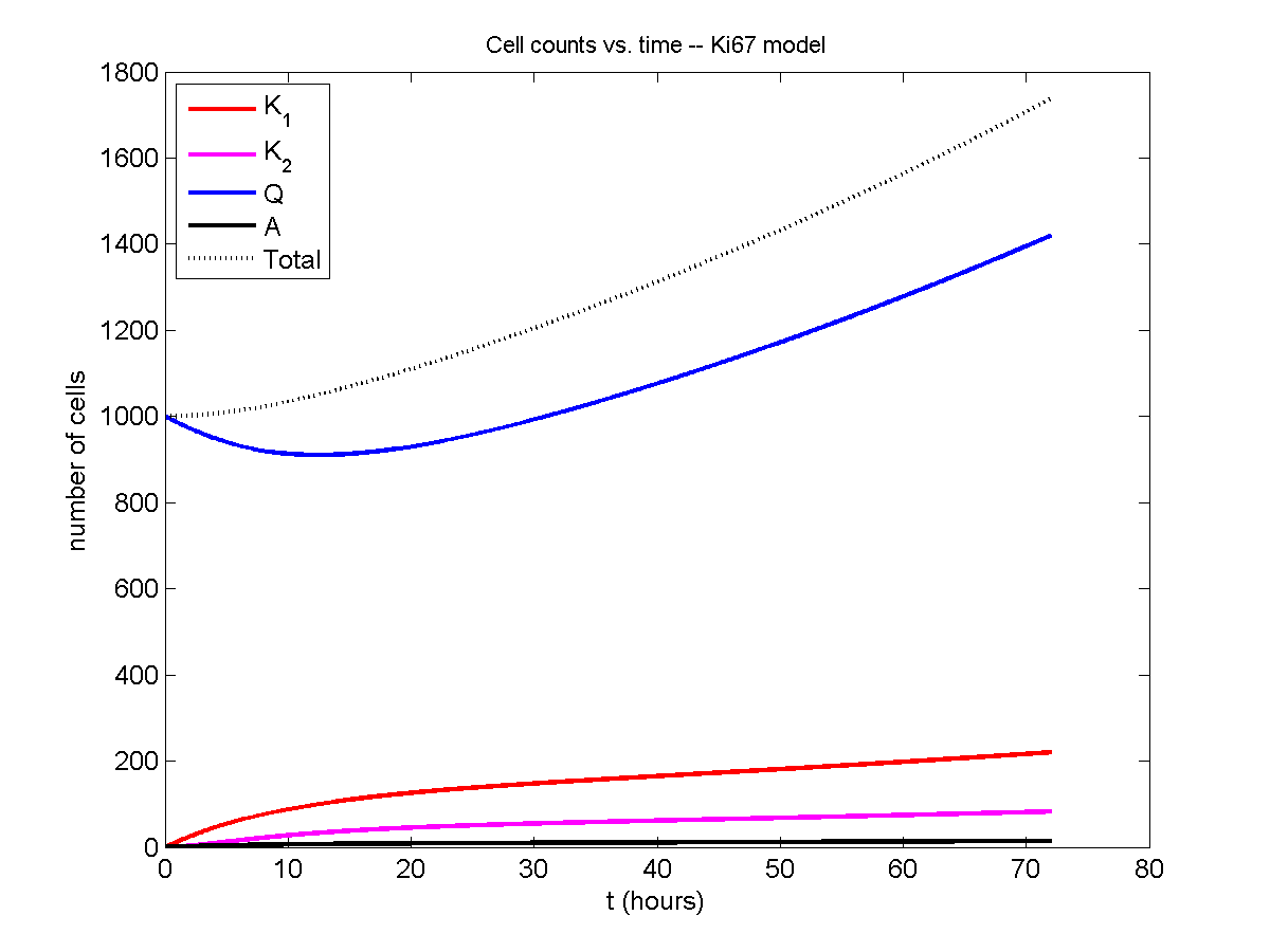
Now, let’s run it and see what this thing looks like:
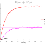
Next, we plot KI1, KI2, and AI versus time (solid curves), along with the theoretical long-time behavior (dashed curves). Notice how well it matches–it’s neat when theory works! :-)
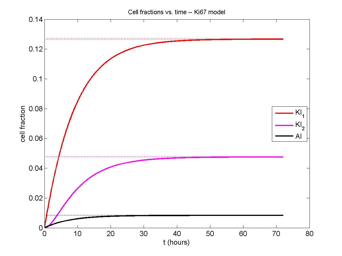
Some readers may recognize the long-time fractions: KI1 + KI2 = KI = 0.1743, and AI = 0.00833, very close to the DCIS patient values from our simulation study in Macklin et al. (2012) and improved calibration work in Hyun and Macklin (2013).
Comparing simulations and theory
I wrote a small Matlab program to implement the discrete model: start with 1000 cells in the \(Q\) phase, and in each time interval \([t,t+\Delta t]\), each cell “decides” whether to advance to the next phase, stay in the same phase, or apoptose. If we compare a single run against the theoretical curves, we see hints of a match:
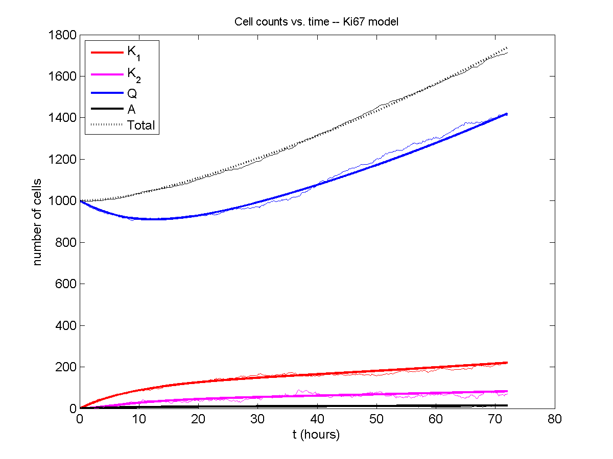
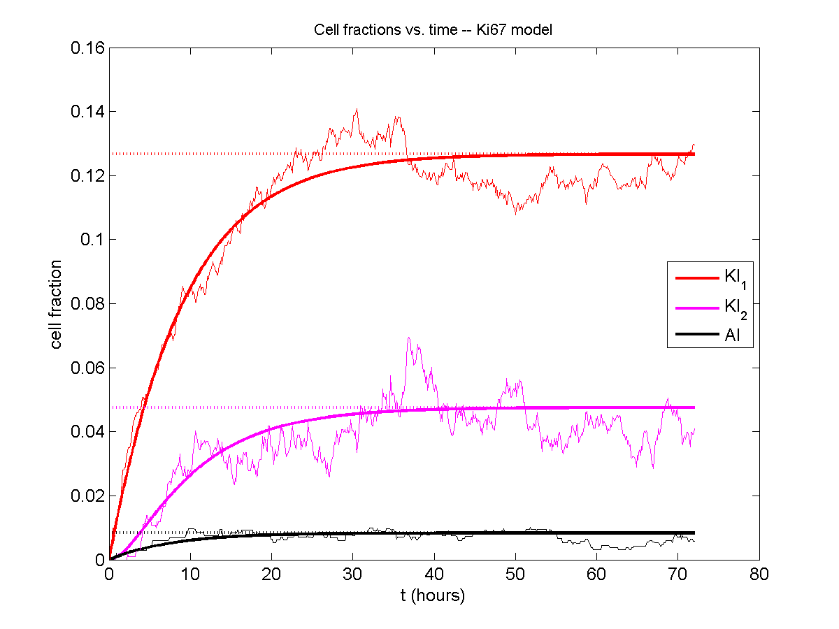
If we average 10 simulations and compare, the match is better:

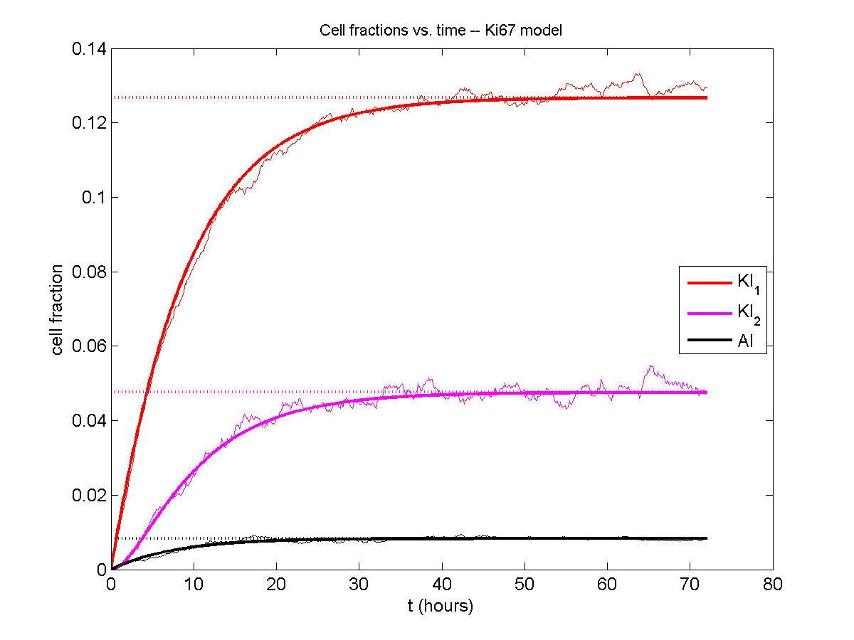
And lastly, if we average 100 simulations and compare, the curves are very difficult to tell apart:
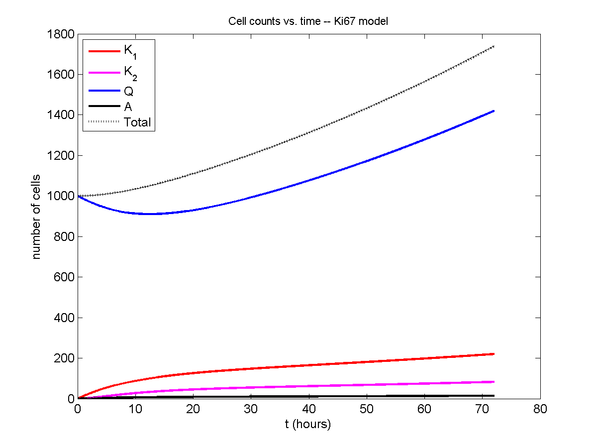

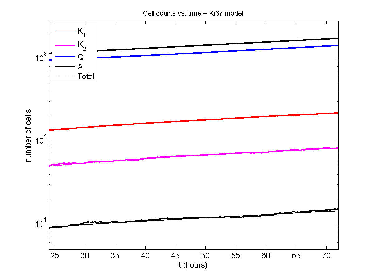
Even in logarithmic space, it’s tough to tell these apart:
Code
The following matlab files (available here) can be used to reproduce this post:
- Ki67_exact.m
- The function defined above to create the exact solution using the eigenvalue/eignvector approach.
- Ki67_stochastic.m
- Runs a single stochastic simulation, using the supplied parameters.
- script.m
- Runs the theoretical solution first, creates plots, and then runs the stochastic model 100 times for comparison.
To make it all work, simply run “script” at the command prompt. Please note that it will generate some png files in its directory.
Closing thoughts
In this post, we showed a nice way to check a discrete model against theoretical behavior–both in short-term dynamics and long-time behavior. The same work should apply to validating many discrete models. However, when you add spatial effects (e.g., a cellular automaton model that won’t proliferate without an empty neighbor site), I wouldn’t expect a match. (But simulating cells that initially have a “salt and pepper”, random distribution should match this for early times.)
Moreover, models with deterministic phase durations (e.g., K1, K2, and A have fixed durations) aren’t consistent with the ODE model above, unless the cells they are each initialized with a random amount of “progress” in their initial phases. (Otherwise, the cells in each phase will run synchronized, and there will be fixed delays before cells transition to other phases.) Delay differential equations better describe such models. However, for long simulation times, the slopes of the sub-populations and the cell fractions should start to better and better match the ODE models.
Now that we have verified that the discrete model is performing as expected, we can have greater confidence in its predictions, and start using those predictions to assess the underlying models. In ODE and PDE models, you often validate the code on simpler problems where you have an analytical solution, and then move on to making simulation predictions in cases where you can’t solve analytically. Similarly, we can now move on to variants of the discrete model where we can’t as easily match ODE theory (e.g., time-varying rate parameters, spatial effects), but with the confidence that the phase transitions are working as they should.
Some quick math to calculate numerical convergence rates
I find myself needing to re-derive this often enough that it’s worth jotting down for current and future students. :-)
Introduction
A very common task in our field is to assess the convergence rate of a numerical algorithm: if I shrink \(\Delta t\) (or \(\Delta x\)), how quickly does my error shrink? And in fact, does my error shrink? Assuming you have a method to compute the error for a simulation (say, a simple test case where you know the exact solution), you want a fit an expression like this:
\[ \mathrm{Error}(\Delta t) = C \Delta t^n ,\] where \( C\) is a constant, and \( n \) is the order of convergence. Usually, if \( n \) isn’t at least 1, it’s bad.
So, suppose you are testing an algorithm, and you have the error \( E_1 \) for \( \Delta t_1 \) and \( E_2 \) for \( \Delta t_2 \). Then one way to go about this calculation is to try to cancel out \( C\):
\begin{eqnarray} \frac{ E_1}{E_2} = \frac{C \Delta t_1^n }{C \Delta t_2^n } = \left( \frac{ \Delta t_1 }{\Delta t_2} \right)^n & \Longrightarrow & n = \frac{ \log\left( E_1 / E_2 \right) }{ \log\left( \Delta t_1 / \Delta t_2 \right) } \end{eqnarray}
Another way to look at this problem is to rewrite the error equation in log-log space:
\begin{eqnarray} E = C \Delta t^N & \Longrightarrow & \log{E} = \log{C} + n \log{ \Delta t} \end{eqnarray}
so \(n\) is the slope of the equation in log space. If you only have two points, then,
\[ n = \frac{ \log{E_1} – \log{E_2} }{ \log{\Delta t_1} – \log{\Delta t_1} } = \frac{ \log\left( E_1 / E_2 \right) }{ \log\left( \Delta t_1 / \Delta t_2 \right) }, \] and so we end up with the exact same convergence rate as before.
However, if you have calculated the error \( E_i \) for a whole bunch of values \( \Delta t_i \), then you can extend this idea to get a better sense of the overall convergence rate for all your values of \( \Delta t \), rather than just two values. Just find the linear least squares fit to the points \( \left\{ ( \log\Delta t_i, \log E_i ) \right\} \). If there are just two points, it’s the same as above. If there are many, it’s a better representation of overall convergence.
Trying it out
Let’s demonstrate this on a simple test problem:
\[ \frac{du}{dt} = -10 u, \hspace{.5in} u(0) = 1.\]
We’ll simulate using (1st-order) forward Euler and (2nd-order) Adams-Bashforth:
dt_vals = [.2 .1 .05 .01 .001 .0001];

min_t = 0;
max_t = 1;

lambda = 10;
initial = 1;

errors_forward_euler = [];
errors_adams_bashforth = [];

for j=1:length( dt_vals )
    dt = dt_vals(j);
    T = min_t:dt:max_t;

    % allocate memory

    solution_forward_euler = zeros(1,length(T));
    solution_forward_euler(1) = initial;
    solution_adams_bashforth = solution_forward_euler;

    % exact solution

    solution_exact = initial * exp( -lambda * T );

    % forward euler

    for i=2:length(T)
        solution_forward_euler(i) = solution_forward_euler(i-1)...
            - dt*lambda*solution_forward_euler(i-1);
    end

    % adams-bashforth -- use high-res Euler to jump-start

    dt_fine = dt * 0.1;
    t = min_t + dt_fine;
    temp = initial ;
    for i=1:10
        temp = temp - dt_fine*lambda*temp;
    end
    solution_adams_bashforth(2) = temp;

    for i=3:length(T)
        solution_adams_bashforth(i) = solution_adams_bashforth(i-1)...
            - 0.5*dt*lambda*( 3*solution_adams_bashforth(i-1)...
            - solution_adams_bashforth(i-2 ) );
    end

%     Uncomments if you want to see plots.
%     figure(1)
%     clf;
%     plot( T, solution_exact, 'r*' , T , solution_forward_euler,...
%         'b-o', T , solution_adams_bashforth , 'k-s'  );
%     pause ;

    errors_forward_euler(j) = ...
        max(abs( solution_exact - solution_forward_euler ) );
    errors_adams_bashforth(j) = ...
        max(abs( solution_exact - solution_adams_bashforth ) );

end
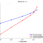
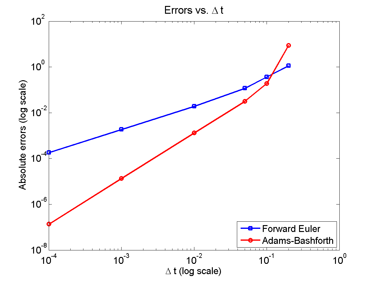
Here is a plot of the errors:
figure(2)
loglog( dt_vals, errors_forward_euler, 'b-s' ,...
    dt_vals, errors_adams_bashforth, 'r-o' ,...
    'linewidth', 2 );
legend( 'Forward Euler', 'Adams-Bashforth' , 4 );
xlabel( '\Delta t (log scale)' , 'fontsize', 14 );
ylabel( 'Absolute errors (log scale)', 'fontsize', 14 );
title( 'Errors vs. \Delta t', 'fontsize' , 16 );
set( gca, 'fontsize' , 14 );
Note that calculating the convergence rate based on the first two errors, and first and last errors, is not terribly
representative, compared with using all the errors:
% Convergence rate based on the first two errors
polyfit( log(dt_vals(1:2)) , log(errors_forward_euler(1:2)) , 1 )
polyfit( log(dt_vals(1:2)) , log(errors_adams_bashforth(1:2)) , 1 )

% Convergence rate based on the first and last errors
m = length(dt_vals);
polyfit( log( [dt_vals(1),dt_vals(m)] ) ,...
    log( [errors_forward_euler(1),errors_forward_euler(m)]) , 1 )
polyfit( log( [dt_vals(1),dt_vals(m)] ) ,...
    log( [errors_adams_bashforth(1),errors_adams_bashforth(m)]) , 1 )

% Convergence rate based on all the errors
polyfit( log(dt_vals) , log(errors_forward_euler) , 1 )
polyfit( log(dt_vals) , log(errors_adams_bashforth) , 1 )

% Convergence rate based on all the errors but the outlier
polyfit( log(dt_vals(2:m)) , log(errors_forward_euler(2:m)) , 1 )
polyfit( log(dt_vals(2:m)) , log(errors_adams_bashforth(2:m)) , 1 )
Using the first two errors gives a convergence rate over 5 for Adams-Bashforth, and around 1.6 for forward Euler. Using first and last is better, but still over-estimates the convergence rates (1.15 and 2.37, FE and AB, respectively). Linear least squares is closer to reality: 1.12 for FE, 2.21 for AB. And lastly, linear least squares but excluding the outliers, we get 1.08 for forward Euler, and 2.03 for Adams-Bashforth. (As expected!)
Which convergence rates are “right”?
So, which values do you report as your convergence rates? Ideally, use all the errors to avoid bias and/or cherry-picking. It’s the most honest and straightforward way to present the work. However, you may have a good rationale to exclude the clear outliers in this case. But then again, if you have calculated the errors for enough values of \(\Delta t\), there’s no need to do this at all. There’s little value in (or basis for) reporting the convergence rate to three significant digits. I’d instead report these as approximately first-order convergence (forward Euler) and approximately second-order convergence (Adams-Bashforth); we get this result with either linear least squares fit, and using all your data points puts you on more solid ground.
Return to News • Return to MathCancer • Follow @MathCancer
Building a Cellular Automaton Model Using BioFVM
Note: This is part of a series of “how-to” blog posts to help new users and developers of BioFVM. See below for guides to setting up a C++ compiler in Windows or OSX.
What you’ll need
- A working C++ development environment with support for OpenMP. See these prior tutorials if you need help.
- A download of BioFVM, available at http://BioFVM.MathCancer.org and http://BioFVM.sf.net. Use Version 1.1.4 or later.
- The source code for this project (see below).
Matlab or Octave for visualization. Matlab might be available for free at your university. Octave is open source and available from a variety of sources.
Our modeling task
We will implement a basic 3-D cellular automaton model of tumor growth in a well-mixed fluid, containing oxygen pO2 (mmHg) and a drug c (e.g., doxorubicin, μM), inspired by modeling by Alexander Anderson, Heiko Enderling, Jan Poleszczuk, Gibin Powathil, and others. (I highly suggest seeking out the sophisticated cellular automaton models at Moffitt’s Integrated Mathematical Oncology program!) This example shows you how to extend BioFVM into a new cellular automaton model. I’ll write a similar post on how to add BioFVM into an existing cellular automaton model, which you may already have available.
Tumor growth will be driven by oxygen availability. Tumor cells can be live, apoptotic (going through energy-dependent cell death, or necrotic (undergoing death from energy collapse). Drug exposure can both trigger apoptosis and inhibit cell cycling. We will model this as growth into a well-mixed fluid, with pO2 = 38 mmHg (about 5% oxygen: a physioxic value) and c = 5 μM.
Mathematical model
As a cellular automaton model, we will divide 3-D space into a regular lattice of voxels, with length, width, and height of 15 μm. (A typical breast cancer cell has radius around 9-10 μm, giving a typical volume around 3.6×103 μm3. If we make each lattice site have the volume of one cell, this gives an edge length around 15 μm.)
In voxels unoccupied by cells, we approximate a well-mixed fluid with Dirichlet nodes, setting pO2 = 38 mmHg, and initially setting c = 0. Whenever a cell dies, we replace it with an empty automaton, with no Dirichlet node. Oxygen and drug follow the typical diffusion-reaction equations:
\[ \frac{ \partial \textrm{pO}_2 }{\partial t} = D_\textrm{oxy} \nabla^2 \textrm{pO}_2 – \lambda_\textrm{oxy} \textrm{pO}_2 – \sum_{ \textrm{cells} i} U_{i,\textrm{oxy}} \textrm{pO}_2 \]
\[ \frac{ \partial c}{ \partial t } = D_c \nabla^2 c – \lambda_c c – \sum_{\textrm{cells }i} U_{i,c} c \]
where each uptake rate is applied across the cell’s volume. We start the treatment by setting c = 5 μM on all Dirichlet nodes at t = 504 hours (21 days). For simplicity, we do not model drug degradation (pharmacokinetics), to approximate the in vitro conditions.
In any time interval [t,t+Δt], each live tumor cell i has a probability pi,D of attempting division, probability pi,A of apoptotic death, and probability pi,N of necrotic death. (For simplicity, we ignore motility in this version.) We relate these to the birth rate bi, apoptotic death rate di,A, and necrotic death rate di,N by the linearized equations (from Macklin et al. 2012):
\[ \textrm{Prob} \Bigl( \textrm{cell } i \textrm{ becomes apoptotic in } [t,t+\Delta t] \Bigr) = 1 – \textrm{exp}\Bigl( -d_{i,A}(t) \Delta t\Bigr) \approx d_{i,A}\Delta t \]
\[ \textrm{Prob} \Bigl( \textrm{cell } i \textrm{ attempts division in } [t,t+\Delta t] \Bigr) = 1 – \textrm{exp}\Bigl( -b_i(t) \Delta t\Bigr) \approx b_{i}\Delta t \]
\[ \textrm{Prob} \Bigl( \textrm{cell } i \textrm{ becomes necrotic in } [t,t+\Delta t] \Bigr) = 1 – \textrm{exp}\Bigl( -d_{i,N}(t) \Delta t\Bigr) \approx d_{i,N}\Delta t \]
\[ \textrm{Prob} \Bigl( \textrm{dead cell } i \textrm{ lyses in } [t,t+\Delta t] \Bigr) = 1 – \textrm{exp}\Bigl( -\frac{1}{T_{i,D}} \Delta t\Bigr) \approx \frac{ \Delta t}{T_{i,D}} \]
(Illustrative) parameter values
We use Doxy = 105 μm2/min (Ghaffarizadeh et al. 2016), and we set Ui,oxy = 20 min-1 (to give an oxygen diffusion length scale of about 70 μm, with steeper gradients than our typical 100 μm length scale). We set λoxy = 0.01 min-1 for a 1 mm diffusion length scale in fluid.
We set Dc = 300 μm2/min, and Uc = 7.2×10⁻³ min-1 (Dc from Weinberg et al. (2007), and Ui,c twice as large as the reference value in Weinberg et al. (2007) to get a smaller diffusion length scale of about 204 μm). We set λc = 3.6×10⁻⁵ min-1 to give a drug diffusion length scale of about 2.9 mm in fluid.
We use TD = 8.6 hours for apoptotic cells, and TD = 60 days for necrotic cells (Macklin et al., 2013). However, note that necrotic and apoptotic cells lose volume quickly, so one may want to revise those time scales to match the point where a cell loses 90% of its volume.
Functional forms for the birth and death rates
We model pharmacodynamics with an area-under-the-curve (AUC) type formulation. If c(t) is the drug concentration at any cell i‘s location at time t, then let its integrated exposure Ei(t) be
\[ E_i(t) = \int_0^t c(s) \: ds \]
and we model its response with a Hill function
\[ R_i(t) = \frac{ E_i^h(t) }{ \alpha_i^h + E_i^h(t) }, \]
where h is the drug’s Hill exponent for the cell line, and α is the exposure for a half-maximum effect.
We model the microenvironment-dependent birth rate by:
\[ b_i(t) = \left\{ \begin{array}{lr} b_{i,P} \left( 1 – \eta_i R_i(t) \right) & \textrm{ if } \textrm{pO}_{2,P} < \textrm{pO}_2 \\ \\ b_{i,P} \left( \frac{\textrm{pO}_{2}-\textrm{pO}_{2,N}}{\textrm{pO}_{2,P}-\textrm{pO}_{2,N}}\right) \Bigl( 1 – \eta_i R_i(t) \Bigr) & \textrm{ if } \textrm{pO}_{2,N} < \textrm{pO}_2 \le \textrm{pO}_{2,P} \\ \\ 0 & \textrm{ if } \textrm{pO}_2 \le \textrm{pO}_{2,N}\end{array} \right. \]
where pO2,P is the physioxic oxygen value (38 mmHg), and pO2,N is a necrotic threshold (we use 5 mmHg), and 0 < η < 1 the drug’s birth inhibition. (A fully cytostatic drug has η = 1.)
We model the microenvironment-dependent apoptosis rate by:
\[ d_{i,A}(t) = d_{i,A}^* + \Bigl( d_{i,A}^\textrm{max} – d_{i,A}^* \Bigr) R_i(t) \]
\[ d_{i,N}(t) = \left\{ \begin{array}{lr} 0 & \textrm{ if } \textrm{pO}_{2,N} < \textrm{pO}_{2} \\ \\ d_{i,N}^* & \textrm{ if } \textrm{pO}_{2} \le \textrm{pO}_{2,N} \end{array}\right. \]
(Illustrative) parameter values
We use bi,P = 0.05 hour-1 (for a 20 hour cell cycle in physioxic conditions), di,A* = 0.01 bi,P, and di,N* = 0.04 hour-1 (so necrotic cells survive around 25 hours in low oxygen conditions).
We set α = 30 μM*hour (so that cells reach half max response after 6 hours’ exposure at a maximum concentration c = 5 μM), h = 2 (for a smooth effect), η = 0.25 (so that the drug is partly cytostatic), and di,Amax = 0.1 hour^-1 (so that cells survive about 10 hours after reaching maximum response).
Building the Cellular Automaton Model in BioFVM
BioFVM already includes Basic_Agents for cell-based substrate sources and sinks. We can extend these basic agents into full-fledged automata, and then arrange them in a lattice to create a full cellular automata model. Let’s sketch that out now.
Extending Basic_Agents to Automata
The main idea here is to define an Automaton class which extends (and therefore includes) the Basic_Agent class. This will give each Automaton full access to the microenvironment defined in BioFVM, including the ability to secrete and uptake substrates. We also make sure each Automaton “knows” which microenvironment it lives in (contains a pointer pMicroenvironment), and “knows” where it lives in the cellular automaton lattice. (More on that in the following paragraphs.)
So, as a schematic (just sketching out the most important members of the class):
class Standard_Data; // define per-cell biological data, such as phenotype,
	// cell cycle status, etc..
class Custom_Data; // user-defined custom data, specific to a model.

class Automaton : public Basic_Agent
{
	private:
		Microenvironment* pMicroenvironment;

		CA_Mesh* pCA_mesh;
		int voxel_index;

	protected:
	public:
		// neighbor connectivity information
		std::vector<Automaton*> neighbors;
		std::vector<double> neighbor_weights;

		Standard_Data standard_data;
		void (*current_state_rule)( Automaton& A , double );

		Automaton();
		void copy_parameters( Standard_Data& SD  );
		void overwrite_from_automaton( Automaton& A );

		void set_cellular_automaton_mesh( CA_Mesh* pMesh );
		CA_Mesh* get_cellular_automaton_mesh( void ) const;

		void set_voxel_index( int );
		int get_voxel_index( void ) const;

		void set_microenvironment( Microenvironment* pME );
		Microenvironment* get_microenvironment( void );

		// standard state changes
		bool attempt_division( void );
		void become_apoptotic( void );
		void become_necrotic( void );
		void perform_lysis( void );

		// things the user needs to define

		Custom_Data custom_data;

		// use this rule to add custom logic
		void (*custom_rule)( Automaton& A , double);
};
So, the Automaton class includes everything in the Basic_Agent class, some Standard_Data (things like the cell state and phenotype, and per-cell settings), (user-defined) Custom_Data, basic cell behaviors like attempting division into an empty neighbor lattice site, and user-defined custom logic that can be applied to any automaton. To avoid lots of switch/case and if/then logic, each Automaton has a function pointer for its current activity (current_state_rule), which can be overwritten any time.
Each Automaton also has a list of neighbor Automata (their memory addresses), and weights for each of these neighbors. Thus, you can distance-weight the neighbors (so that corner elements are farther away), and very generalized neighbor models are possible (e.g., all lattice sites within a certain distance). When updating a cellular automaton model, such as to kill a cell, divide it, or move it, you leave the neighbor information alone, and copy/edit the information (standard_data, custom_data, current_state_rule, custom_rule). In many ways, an Automaton is just a bucket with a cell’s information in it.
Note that each Automaton also “knows” where it lives (pMicroenvironment and voxel_index), and knows what CA_Mesh it is attached to (more below).
Connecting Automata into a Lattice
An automaton by itself is lost in the world–it needs to link up into a lattice organization. Here’s where we define a CA_Mesh class, to hold the entire collection of Automata, setup functions (to match to the microenvironment), and two fundamental operations at the mesh level: copying automata (for cell division), and swapping them (for motility). We have provided two functions to accomplish these tasks, while automatically keeping the indexing and BioFVM functions correctly in sync. Here’s what it looks like:
class CA_Mesh{
	private:
		Microenvironment* pMicroenvironment;
		Cartesian_Mesh* pMesh;

		std::vector<Automaton> automata;
		std::vector<int> iteration_order;
	protected:
	public:
		CA_Mesh();

		// setup to match a supplied microenvironment
		void setup( Microenvironment& M );
		// setup to match the default microenvironment
		void setup( void );

		int number_of_automata( void ) const;

		void randomize_iteration_order( void );

		void swap_automata( int i, int j );
		void overwrite_automaton( int source_i, int destination_i );

		// return the automaton sitting in the ith lattice site
		Automaton& operator[]( int i );

		// go through all nodes according to random shuffled order
		void update_automata( double dt );
};
So, the CA_Mesh has a vector of Automata (which are never themselves moved), pointers to the microenvironment and its mesh, and a vector of automata indices that gives the iteration order (so that we can sample the automata in a random order). You can easily access an automaton with operator[], and copy the data from one Automaton to another with overwrite_automaton() (e.g, for cell division), and swap two Automata’s data (e.g., for cell migration) with swap_automata(). Finally, calling update_automata(dt) iterates through all the automata according to iteration_order, calls their current_state_rules and custom_rules, and advances the automata by dt.
Interfacing Automata with the BioFVM Microenvironment
The setup function ensures that the CA_Mesh is the same size as the Microenvironment.mesh, with same indexing, and that all automata have the correct volume, and dimension of uptake/secretion rates and parameters. If you declare and set up the Microenvironment first, all this is take care of just by declaring a CA_Mesh, as it seeks out the default microenvironment and sizes itself accordingly:
// declare a microenvironment
Microenvironment M;
// do things to set it up -- see prior tutorials
// declare a Cellular_Automaton_Mesh
CA_Mesh CA_model;
// it's already good to go, initialized to empty automata:
CA_model.display();
If you for some reason declare the CA_Mesh fist, you can set it up against the microenvironment:
// declare a CA_Mesh
CA_Mesh CA_model;
// declare a microenvironment
Microenvironment M;
// do things to set it up -- see prior tutorials
// initialize the CA_Mesh to match the microenvironment
CA_model.setup( M );
// it's already good to go, initialized to empty automata:
CA_model.display();
Because each Automaton is in the microenvironment and inherits functions from Basic_Agent, it can secrete or uptake. For example, we can use functions like this one:
void set_uptake( Automaton& A, std::vector<double>& uptake_rates )
{
extern double BioFVM_CA_diffusion_dt;
// update the uptake_rates in the standard_data
A.standard_data.uptake_rates = uptake_rates;
// now, transfer them to the underlying Basic_Agent
*(A.uptake_rates) = A.standard_data.uptake_rates;
// and make sure the internal constants are self-consistent
A.set_internal_uptake_constants( BioFVM_CA_diffusion_dt );
}
A function acting on an automaton can sample the microenvironment to change parameters and state. For example:
void do_nothing( Automaton& A, double dt )
{ return; }

void microenvironment_based_rule( Automaton& A, double dt )
{
	// sample the microenvironment
	std::vector<double> MS = (*A.get_microenvironment())( A.get_voxel_index() );

	// if pO2 < 5 mmHg, set the cell to a necrotic state
	if( MS[0] < 5.0 ) { A.become_necrotic(); } // if drug > 5 uM, set the birth rate to zero
	if( MS[1] > 5 )
	{ A.standard_data.birth_rate = 0.0; }

	// set the custom rule to something else
	A.custom_rule = do_nothing;

	return;
}
Implementing the mathematical model in this framework
We give each tumor cell a tumor_cell_rule (using this for custom_rule):
void viable_tumor_rule( Automaton& A, double dt )
{
	// If there's no cell here, don't bother.
	if( A.standard_data.state_code == BioFVM_CA_empty )
	{ return; }

	// sample the microenvironment
	std::vector<double> MS = (*A.get_microenvironment())( A.get_voxel_index() );

	// integrate drug exposure
	A.standard_data.integrated_drug_exposure += ( MS[1]*dt );
	A.standard_data.drug_response_function_value = pow( A.standard_data.integrated_drug_exposure,
		A.standard_data.drug_hill_exponent );
	double temp = pow( A.standard_data.drug_half_max_drug_exposure,
		A.standard_data.drug_hill_exponent );
	temp += A.standard_data.drug_response_function_value;
	A.standard_data.drug_response_function_value /= temp;

	// update birth rates (which themselves update probabilities)
	update_birth_rate( A, MS, dt );
	update_apoptotic_death_rate( A, MS, dt );
	update_necrotic_death_rate( A, MS, dt );

	return;
}
The functional tumor birth and death rates are implemented as:
void update_birth_rate( Automaton& A, std::vector<double>& MS, double dt )
{
	static double O2_denominator = BioFVM_CA_physioxic_O2 - BioFVM_CA_necrotic_O2;

	A.standard_data.birth_rate = 	A.standard_data.drug_response_function_value;
		// response
	A.standard_data.birth_rate *= A.standard_data.drug_max_birth_inhibition;
		// inhibition*response;
	A.standard_data.birth_rate *= -1.0;
		// - inhibition*response
	A.standard_data.birth_rate += 1.0;
		// 1 - inhibition*response
	A.standard_data.birth_rate *= viable_tumor_cell.birth_rate;
		// birth_rate0*(1 - inhibition*response)

	double temp1 = MS[0] ; // O2
	temp1 -= BioFVM_CA_necrotic_O2;
	temp1 /= O2_denominator;

	A.standard_data.birth_rate *= temp1;
	if( A.standard_data.birth_rate < 0 )
	{ A.standard_data.birth_rate = 0.0; }

	A.standard_data.probability_of_division = A.standard_data.birth_rate;
	A.standard_data.probability_of_division *= dt;
		// dt*birth_rate*(1 - inhibition*repsonse) // linearized probability
	return;
}

void update_apoptotic_death_rate( Automaton& A, std::vector<double>& MS, double dt )
{
	A.standard_data.apoptotic_death_rate = A.standard_data.drug_max_death_rate;
		// max_rate
	A.standard_data.apoptotic_death_rate -= viable_tumor_cell.apoptotic_death_rate;
		// max_rate - background_rate
	A.standard_data.apoptotic_death_rate *= A.standard_data.drug_response_function_value;
		// (max_rate-background_rate)*response
	A.standard_data.apoptotic_death_rate += viable_tumor_cell.apoptotic_death_rate;
		// background_rate + (max_rate-background_rate)*response

	A.standard_data.probability_of_apoptotic_death = A.standard_data.apoptotic_death_rate;
	A.standard_data.probability_of_apoptotic_death *= dt;
		// dt*( background_rate + (max_rate-background_rate)*response ) // linearized probability
	return;
}

void update_necrotic_death_rate( Automaton& A, std::vector<double>& MS, double dt )
{
	A.standard_data.necrotic_death_rate = 0.0;
	A.standard_data.probability_of_necrotic_death = 0.0;

	if( MS[0] > BioFVM_CA_necrotic_O2 )
	{ return; }

	A.standard_data.necrotic_death_rate = perinecrotic_tumor_cell.necrotic_death_rate;
	A.standard_data.probability_of_necrotic_death = A.standard_data.necrotic_death_rate;
	A.standard_data.probability_of_necrotic_death *= dt;
		// dt*necrotic_death_rate

	return;
}
And each fluid voxel (Dirichlet nodes) is implemented as the following (to turn on therapy at 21 days):
void fluid_rule( Automaton& A, double dt )
{
	static double activation_time = 504;
	static double activation_dose = 5.0;
	static std::vector<double> activated_dirichlet( 2 , BioFVM_CA_physioxic_O2 );
	static bool initialized = false;
	if( !initialized )
	{
		activated_dirichlet[1] = activation_dose;
		initialized = true;
	}

	if( fabs( BioFVM_CA_elapsed_time - activation_time ) < 0.01 ) { int ind = A.get_voxel_index(); if( A.get_microenvironment()->mesh.voxels[ind].is_Dirichlet )
		{
			A.get_microenvironment()->update_dirichlet_node( ind, activated_dirichlet );
		}
	}
}
At the start of the simulation, each non-cell automaton has its custom_rule set to fluid_rule, and each tumor cell Automaton has its custom_rule set to viable_tumor_rule. Here’s how:
void setup_cellular_automata_model( Microenvironment& M, CA_Mesh& CAM )
{
	// Fill in this environment
	double tumor_radius = 150;
	double tumor_radius_squared = tumor_radius * tumor_radius;

	std::vector<double> tumor_center( 3, 0.0 );

	std::vector<double> dirichlet_value( 2 , 1.0 );
	dirichlet_value[0] = 38; //physioxia
	dirichlet_value[1] = 0; // drug

	for( int i=0 ; i < M.number_of_voxels() ;i++ )
	{
		std::vector<double> displacement( 3, 0.0 );
		displacement = M.mesh.voxels[i].center;
		displacement -= tumor_center;
		double r2 = norm_squared( displacement );

		if( r2 > tumor_radius_squared ) // well_mixed_fluid
		{
			M.add_dirichlet_node( i, dirichlet_value );
			CAM[i].copy_parameters( well_mixed_fluid );
			CAM[i].custom_rule = fluid_rule;
			CAM[i].current_state_rule = do_nothing;
		}
		else // tumor
		{
			CAM[i].copy_parameters( viable_tumor_cell );
			CAM[i].custom_rule = viable_tumor_rule;
			CAM[i].current_state_rule = advance_live_state;
		}

	}
}
Overall program loop
There are two inherent time scales in this problem: cell processes like division and death (happen on the scale of hours), and transport (happens on the order of minutes). We take advantage of this by defining two step sizes:
double BioFVM_CA_dt = 3;
std::string BioFVM_CA_time_units = "hr";
double BioFVM_CA_save_interval = 12;
double BioFVM_CA_max_time = 24*28;
double BioFVM_CA_elapsed_time = 0.0;

double BioFVM_CA_diffusion_dt = 0.05;

std::string BioFVM_CA_transport_time_units = "min";
double BioFVM_CA_diffusion_max_time = 5.0;
Every time the simulation advances by BioFVM_CA_dt (on the order of hours), we run diffusion to quasi-steady state (for BioFVM_CA_diffusion_max_time, on the order of minutes), using time steps of size BioFVM_CA_diffusion time. We performed numerical stability and convergence analyses to determine 0.05 min works pretty well for regular lattice arrangements of cells, but you should always perform your own testing!
Here’s how it all looks, in a main program loop:
BioFVM_CA_elapsed_time = 0.0;
double next_output_time = BioFVM_CA_elapsed_time; // next time you save data

while( BioFVM_CA_elapsed_time < BioFVM_CA_max_time + 1e-10 )
{
	// if it's time, save the simulation
	if( fabs( BioFVM_CA_elapsed_time - next_output_time ) < BioFVM_CA_dt/2.0 )
	{
		std::cout << "simulation time: " << BioFVM_CA_elapsed_time << " " << BioFVM_CA_time_units
			<< " (" << BioFVM_CA_max_time << " " << BioFVM_CA_time_units << " max)" << std::endl;
		char* filename;
		filename = new char [1024];
		sprintf( filename, "output_%6f" , next_output_time );
		save_BioFVM_cellular_automata_to_MultiCellDS_xml_pugi( filename , M , CA_model ,
			BioFVM_CA_elapsed_time );

		cell_counts( CA_model );
		delete [] filename;
		next_output_time += BioFVM_CA_save_interval;
	}

	// do the cellular automaton step
	CA_model.update_automata( BioFVM_CA_dt );
	BioFVM_CA_elapsed_time += BioFVM_CA_dt;

	// simulate biotransport to quasi-steady state

	double t_diffusion = 0.0;
	while( t_diffusion < BioFVM_CA_diffusion_max_time + 1e-10 )
	{
		M.simulate_diffusion_decay( BioFVM_CA_diffusion_dt );
		M.simulate_cell_sources_and_sinks( BioFVM_CA_diffusion_dt );
		t_diffusion += BioFVM_CA_diffusion_dt;
	}
}
Getting and Running the Code
- Start a project: Create a new directory for your project (I’d recommend “BioFVM_CA_tumor”), and enter the directory. Place a copy of BioFVM (the zip file) into your directory. Unzip BioFVM, and copy BioFVM*.h, BioFVM*.cpp, and pugixml* files into that directory.
- Download the demo source code: Download the source code for this tutorial: BioFVM_CA_Example_1, version 1.0.0 or later. Unzip its contents into your project directory. Go ahead and overwrite the Makefile.
- Edit the makefile (if needed): Note that if you are using OSX, you’ll probably need to change from “g++” to your installed compiler. See these tutorials.
- Test the code: Go to a command line (see previous tutorials), and test:
make
./BioFVM_CA_Example_1
(If you’re on windows, run BioFVM_CA_Example_1.exe.)
Simulation Result
If you run the code to completion, you will simulate 3 weeks of in vitro growth, followed by a bolus “injection” of drug. The code will simulate one one additional week under the drug. (This should take 5-10 minutes, including full simulation saves every 12 hours.)
In matlab, you can load a saved dataset and check the minimum oxygenation value like this:
MCDS = read_MultiCellDS_xml( 'output_504.000000.xml' );
min(min(min( MCDS.continuum_variables(1).data )))
And then you can start visualizing like this:
contourf( MCDS.mesh.X_coordinates , MCDS.mesh.Y_coordinates , ...
MCDS.continuum_variables(1).data(:,:,33)' ) ;
axis image;
colorbar
xlabel('x (\mum)' , 'fontsize' , 12 );
ylabel( 'y (\mum)' , 'fontsize', 12 );
set(gca, 'fontsize', 12 );
title('Oxygenation (mmHg) at z = 0 \mum', 'fontsize', 14 );
print('-dpng', 'Tumor_o2_3_weeks.png' );
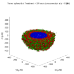
plot_cellular_automata( MCDS , 'Tumor spheroid at 3 weeks');
Simulation plots
Here are some plots, showing (left from right) pO2 concentration, a cross-section of the tumor (red = live cells, green = apoptotic, and blue = necrotic), and the drug concentration (after start of therapy):
1 week:

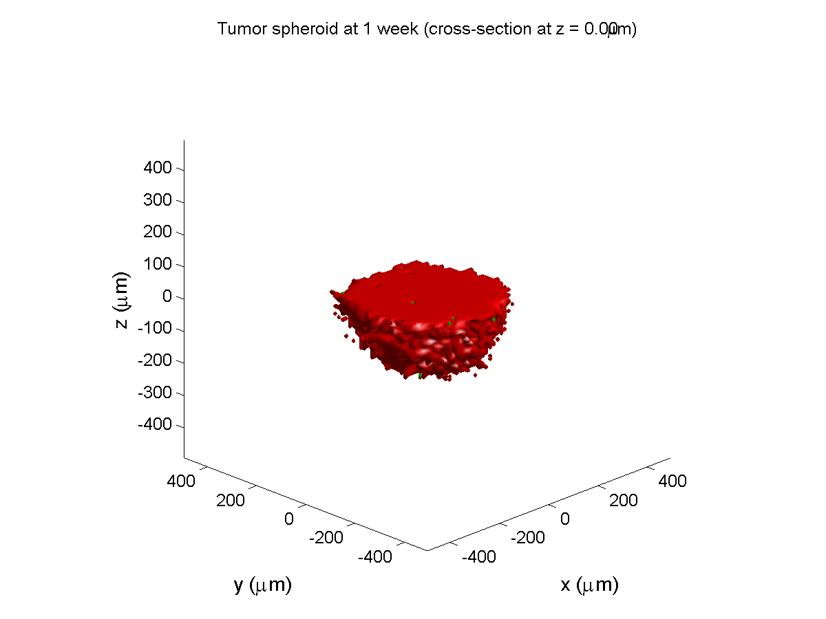
Oxygen- and space-limited growth are restricted to the outer boundary of the tumor spheroid.
2 weeks:
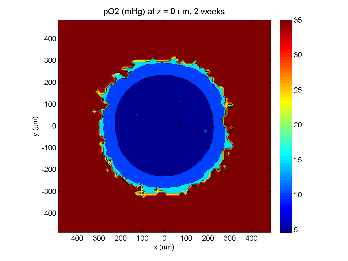
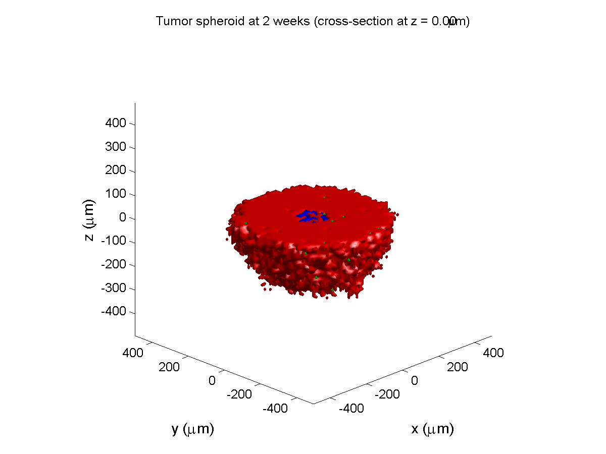
Oxygenation is dipped below 5 mmHg in the center, leading to necrosis.
3 weeks:
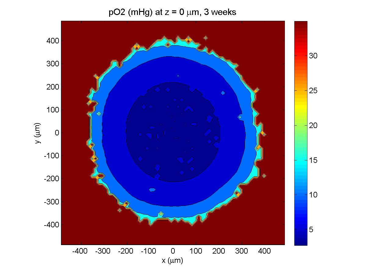
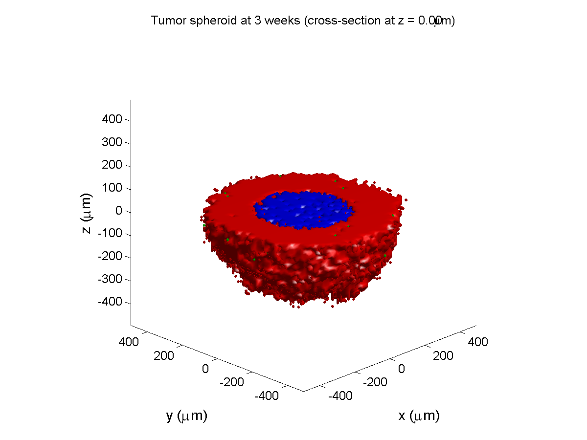
As the tumor grows, the hypoxic gradient increases, and the necrotic core grows. The code turns on a constant 5 micromolar dose of doxorubicin at this point
Treatment + 12 hours:
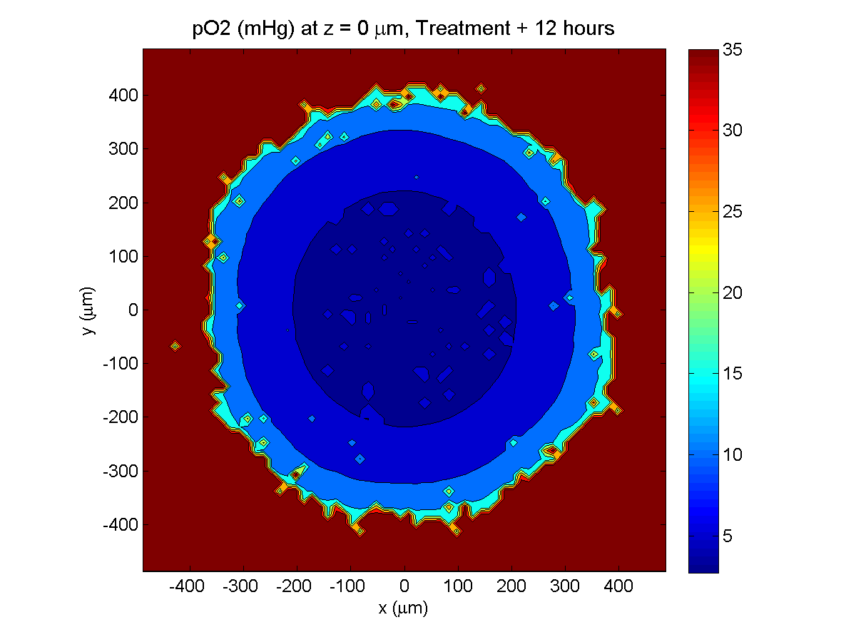
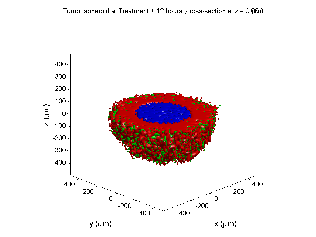

The drug has started to penetrate the tumor, triggering apoptotic death towards the outer periphery where exposure has been greatest.
Treatment + 24 hours:


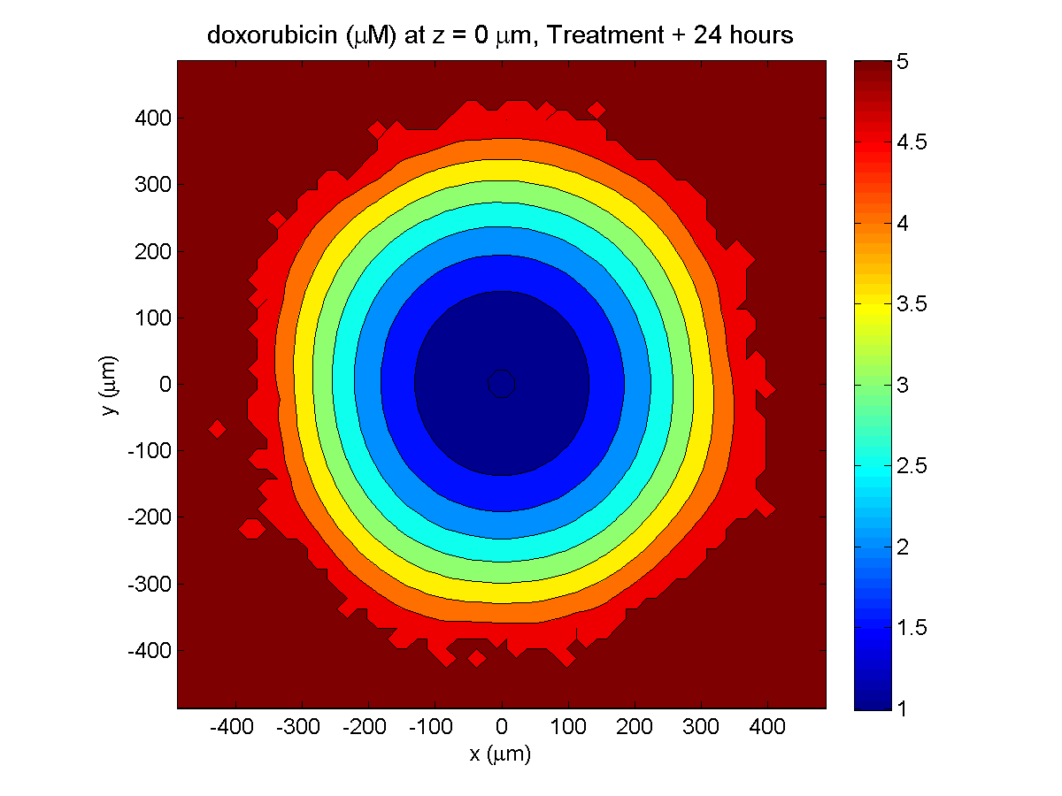
The drug profile hasn’t changed much, but the interior cells have now had greater exposure to drug, and hence greater response. Now apoptosis is observed throughout the non-necrotic tumor. The tumor has decreased in volume somewhat.
Treatment + 36 hours:
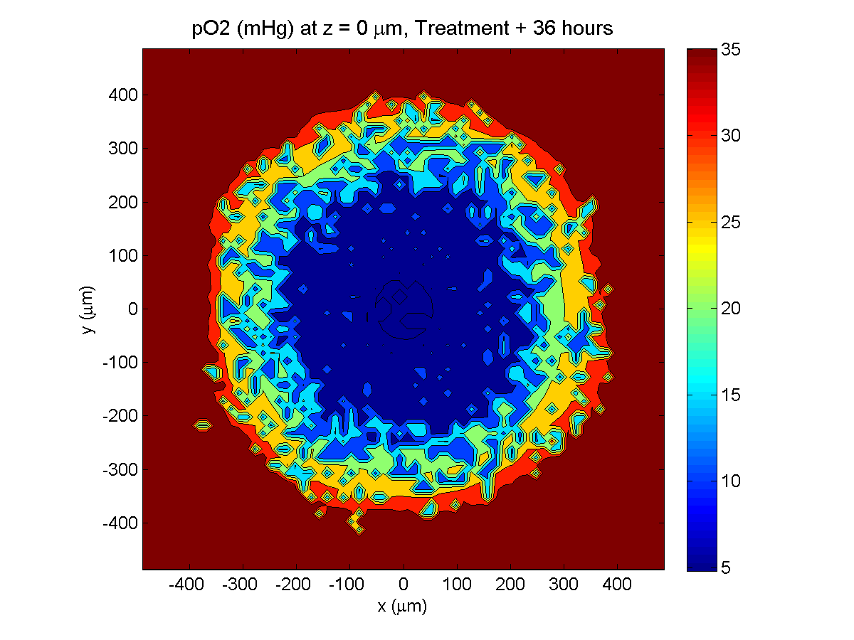
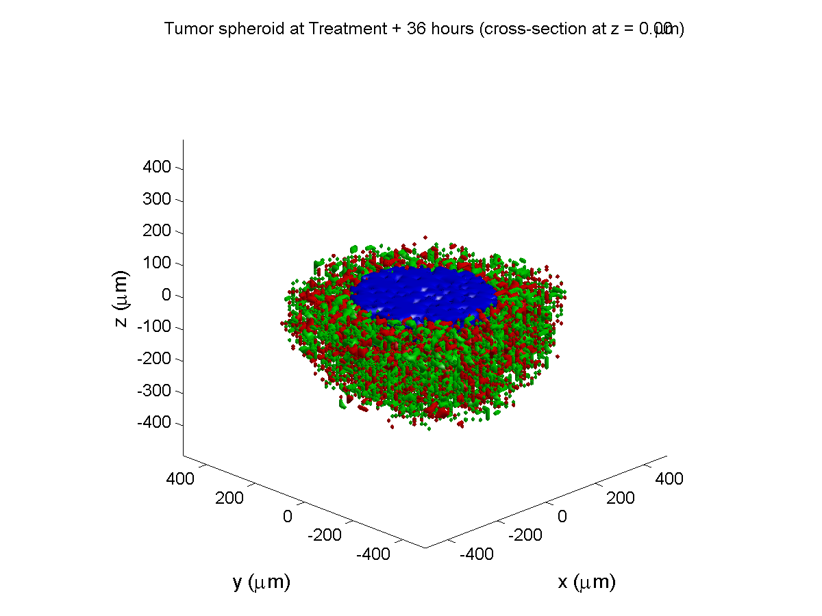
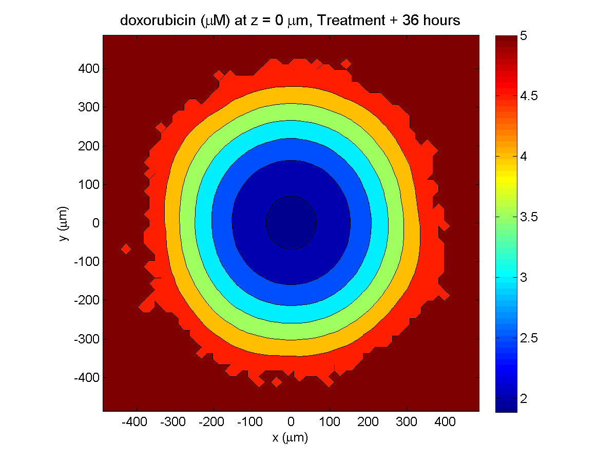
The non-necrotic tumor is now substantially apoptotic. We would require some pharamcokinetic effects (e.g., drug clearance, inactivation, or removal) to avoid the inevitable, presences of a pre-existing resistant strain, or emergence of resistance.
Treatment + 48 hours:
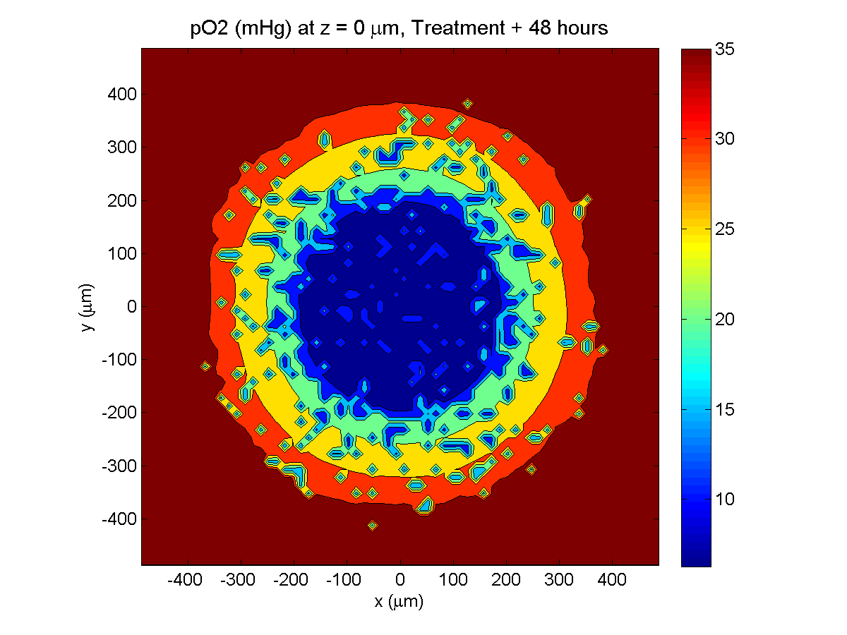
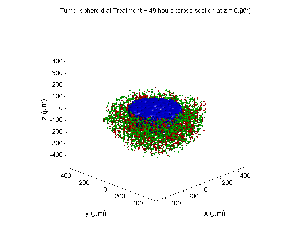
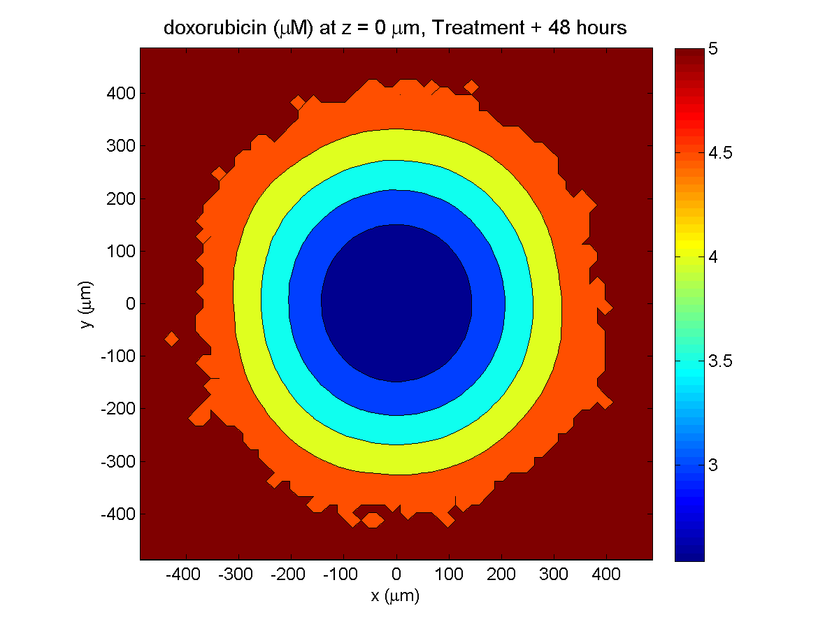
By now, almost all cells are apoptotic.
Treatment + 60 hours:

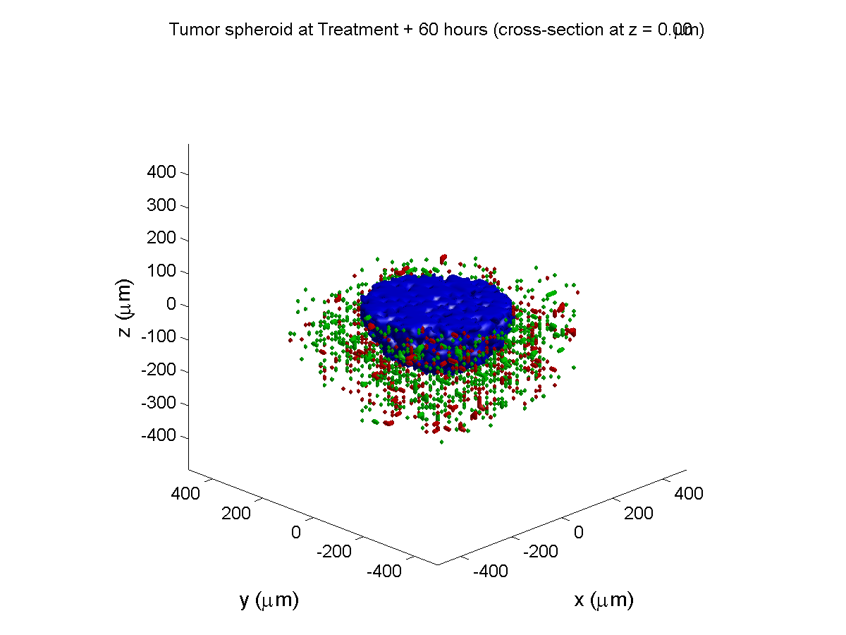

The non-necrotic tumor is nearly completed eliminated, leaving a leftover core of previously-necrotic cells (which did not change state in response to the drug–they were already dead!)
Source files
You can download completed source for this example here: https://sourceforge.net/projects/biofvm/files/Tutorials/Cellular_Automaton_1/
This file will include the following:
- BioFVM_cellular_automata.h
- BioFVM_cellular_automata.cpp
- BioFVM_CA_example_1.cpp
- read_MultiCellDS_xml.m (updated)
- plot_cellular_automata.m
- Makefile
What’s next
I plan to update this source code with extra cell motility, and potentially more realistic parameter values. Also, I plan to more formally separate out the example from the generic cell capabilities, so that this source code can work as a bona fide cellular automaton framework.
More immediately, my next tutorial will use the reverse strategy: start with an existing cellular automaton model, and integrate BioFVM capabilities.
Return to News • Return to MathCancer • Follow @MathCancer
Moving the blog to MathCancer.org
Hi, everyone!
Blogspot has been a great platform for me, but in the end, editing posts with source code and mathematics has been too much of a headache in the neglected blogspot and google UIs.
Elsewhere in the universe, WordPress has developed and encouraged a great ecosystem of plugins that let you do LaTeX and code syntax highlighting directly in your posts with ease. I can’t spend hours and hours on fixing mangled posts. It’s time to move on.
So as of today, I am moving to a self-hosted blog at http://MathCancer.org/blog/
I will leave old posts at http://MathCancer.blogspot.com and gradually migrate them here to MathCancer.org/blog. Thanks for following me over the last few years.
Return to News • Return to MathCancer • Follow @MathCancer
Paul Macklin featured in Biotechniques article
Paul Macklin’s work on mathematical modeling of breast cancer and BioFVM was recently featured in Kelly Rae Chi’s article in Biotechniques on virtual cell cultures. It also included great work by James Glazier (CompuCell3D) and Kristin Swanson (glioblastoma modeling).
Read the article: http://www.biotechniques.com/news/Mighty-Modelers-The-Art-of-Virtual-Cell-Culture/biotechniques-364893.html (July 20, 2016)
Return to News • Return to MathCancer • Follow @MathCancer